Floating Conductor
A floating conductor is a conductor that is not held to a known potential by a connection to electrical ground or a power supply. Rather it is isolated (insulated) from these voltage sources. As a conductor, it still has some constant potential over the entire surface, but you might not know a priori what that potential value is. This potential is not fixed to a known value but rather depends on the surrounding potentials or field, as usually calculated by the Laplace Equation (SIMION Refine process), which circularly depends again on the potential of the floating conductor. What you do, or should, know, however, about the floating conductor is the total charge Q on it (perhaps zero). The total charge on a floating conductor will remain constant if it’s electrically isolated from all sources of charge, such as if it’s held in place by a perfect insulator and no charged particle beam hits it.
There are at least two ways to calculate fields with floating conductors in SIMION. In SIMION 8.1.1.0 or above, which supports dielectrics, floating conductors may be treated as a dielectric material with a large (nearly infinite) dielectric constant. Another way, and the only way in early versions, is to set the surfaces to two arbitrary potentials, apply Gauss’s Law to determine the charge on the conductor at each potential, and then solve for the potential necessary to generate the requisite charge. These methods are described below.
Note
This page is abridged from the full SIMION "Supplemental Documentation" (Help file). The following additional sections can be found in the full version of this page accessible via the "Help > Supplemental Documentation" menu in SIMION 8.1.1 or above:- Modeling as dielectrics
Modeling with the standard Laplace solver
The SIMION refine process prior to 8.1.1.0 does not directly provide for the specification of floating conductors. However, there is still a way to do this calculation in SIMION, at least since version 6.0:
- Model the system with a fast adjust potential array (PA# file). Make the floating conductor a separate fast adjust electrode.
- Refine the PA.
- Fast adjust the non-floating conductors to 0 V and the floating conductor to 1 V. Save the PA0 file and calculate the total charge Q1 on the floating conductor under these conditions as described in Charge-Capacitance Calculation.
- Repeat step #3 but fast adjust the non-floating conductors to appropriate values and the floating conductor to 0V. The calculated total charge will now be named Q2.
- The proper potential Vf on the floating conductor is then found by solving Vf * Q1 + (1 V) * Q2 = Q. This is a direct result from Gauss’s Law given that the actual field is some (unknown) linear combination of the two cases above (i.e. principle of superposition or SIMION fast adjust). (*2) Fast adjust the floating conductor to this potential.
- As an optional check, you may repeat the total charge calculation with the final potentials to confirm that the total charge on the floating conductor is as expected.
This is demonstrated in SIMION Example: gauss_law in SIMION 8.0 (and further simplified in 8.1). There was previously a version of this in the SL Toolkit (prior to the 8.0 release).
An example of this is shown in Figure 1. This is a 2D planar parallel plate system with a floating conductor of zero charge placed in the middle at a 45 degree angle. The parallel plates are at 0V and 1V, and by symmetry alone we predict the floating conductor to be at 0.5V.
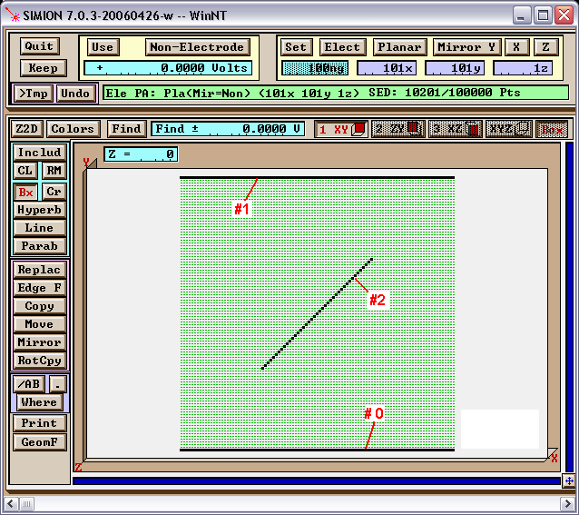
Fig. 59 Figure 1: Setting up the PA in Modify.
In fact, using the “run” program around the perimeter box2d(20,20, 80,80) we obtain integration results of Q1 = 3.3517E-14 and Q2 = -1.6684E-14, and we already know that Q = 0. Solving the linear equation then gives Qf = 0.498 V, roughly as we expect. The resultant potential contours with the floating conductor fast-adjusted to this voltage are shown in Figure 2.

Fig. 60 Figure 2: Viewing the potential contour lines in View. Note: there is a type of vertical symmetry on the field since the charge of the floating conductor (center) is zero.
Other Notes
One practical remark by Marc [*1]–in working with charged particles, floating conductor surfaces will collect particles emitted from the source. This charge capture modifies the potential very fast until the beam is fully repelled. In most cases the floating conductor will finally reach a potential close to the potential of the emitting source. In electrostatic optical systems one should be aware of charge captures on insulating surfaces. Therefore the insulator should as far as possible from the optics’ “active” elements.
Also noted by Frank [*2]–a similar approach has been used in simulating magnetic shields in SIMION. For mu -> infinity materials (“mu metals”), the magnetic potential is constant at the surface. So SIMION’s approach to magnetic fields is quite natural if you know what potential to put on the PAs. Using the same logic above, one can set the potential so that a Gaussian integral around the shield PA is zero, which is the only choice satisfying div B = 0.
- [*1] Marc Bernheim - SIMION User Group Discussion #367 - Floating Conductor
- [*2] Frank Crary - SIMION User Group Discussion #367b - Floating Conductor + SIMION User Group Discussion #633 - Mu-Metal simulation