
Note: this article is older. See Importing and Exporting Field and Potential Array Data for the latest information on newer methods of doing this. In additional, SIMION 8.0 now includes a Biot-Savart solver.
June 2005, David Manura, Scientific Instrument Services, Inc. (Updated Jan 2006)
Abstract
This article describes multiple methods of importing the magnetic field of a solenoid coil into SIMION. Special methods are required because although SIMION can apply a known arbitrary magnetic field to particles, SIMION cannot always calculate that magnetic field directly, e.g. if the problem is not expressible in terms of scalar magnetic potential. SIMION does not directly or exactly calculate, for example, the magnetic fields generated by wire currents and in particular the fringing effects at the ends of a solenoid coil. Therefore, we may rather utilize an external program (CPO), a formula, or even an approximation in terms of scalar magnetic potential and then import that field into SIMION via a SIMION user program or even via a SIMION potential array (PA) file.
Introduction
A schematic of a (finite, thin) solenoid is shown below with its main parameters:
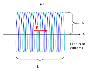
Figure: Schematic of solenoid coil.
A current i is applied through N coils of radius r0 and length L to generate a magnetic field B. The solenoid has an axis of symmetry (we use the x-axis, according to the SIMION convention, but the z-axis is often used elsewhere). B is largely uniform inside the solenoid and near zero outside. As we shall see, this is the ideal case since in practice B is not uniform nor zero near the two sides of the solenoid (the "fringing effects"), and field irregularities occur, though possibly to only a small extent, near the finite width wires themselves.
We first examine the appearance of the solenoid magnetic field and how to calculate it in the CPO software. Then we move on to importing this field data into SIMION or instead using a formula or approximation.
Outline
- Calculating the magnetic field in CPO
- Importing the magnetic field into SIMION:
- Import Method #1: Using a user program (PRG or SL).
- Approach #1.1: Using a formula
- Approach #1.2: Interpolating the grid data
- Import Method #2: Constructing a PA file
- Approach #2.1: Converting the grid data to a PA file using the SL Tools.
- Approach #2.2: Constructing an approximate PA file manually from the grid data with Modify.
- Approach #2.3: Constructing an approximate PA file with the SL Toolkit
- Approach #2.4: Constructing an approximate PA file entirely with Modify.
- Import Method #1: Using a user program (PRG or SL).
What you may need:
- SIMION - the goal is to import the fields into SIMION.
- CPO-3D - Some of the methods here use CPO to calculate the magnetic field.
- SIMION SL Toolkit - Some of the methods here use the SIMION SL Toolkit
to convert the field data into a SIMION PA file.
(Both CPO-3D and SIMION SL are optional, e.g. when using approach #2.4.)
Calculating the magnetic field in CPO
We first seek to calculate the magnetic field of a solenoid coil. Here, we use the CPO software, which is able to calculate magnetic fields generated by arbitrary length of current-carrying wire, such as a solenoid coil.
CPO provides a canned method for defining solenoid coils, so the task is fairly easy. Below is defined a solenoid with simple parameters meant only for demonstration. The coil is centered at the origin and extended +- 2 mm along the z-axis (the z-axis, rather than the x-axis, is conventionally used for the axis in CPO). The coil has radius 1 mm, there are 100 turns of coil, and the current though it is 1 A.

Figure: CPO definition of magnetic solenoid element ("Databuilder | Magnetic Fields").
Upon running the calculation, CPO will solve this magnetic field. The magnetic field vectors, intensities, and contours can be displayed as shown below. The plots are over the x=0 plane, which contains the axis of symmetry.

Figure: CPO plot of magnetic field vectors.

Figure: CPO plot of magnetic field intensities (the red in the center is high intensity).

Figure: CPO plot of magnetic field contour lines.

Figure: Definition of CPO contours lines above: 0, 0.001, ..., 0.035 Tesla. The same contours will be drawn later in SIMION for comparison.
Note that the fields inside the solenoid are fairly uniform. However, the field behaves in a more complicated manner near the two ends (fringing effects).
Just computing the magnetic field above is not enough. We need to get this data in a format that is suitable for import into SIMION. Basically, we want a text file containing the magnetic fields vectors at each point on a rectangular grid. Because of the cylindrical symmetry of the problem, it is sufficient to record the fields on only the positive (x > 0) half of the x=0 plane containing the axis of the symmetry (z). We will confine the region of interest to z in [-4, 4] and x in [0, 2]. We might even consider omitting the negative half of the z-axis due to the antisymmetry of the field (assuming coil spacing is small), but we will not do so since SIMION PA files (which will be generated at least in Method #2 below) do not support antisymmetry on voltages. The configuration of the data recording is shown below.

Figure: CPO definition of recording of fields on 2D grid ("Databuilder | Potentials and Fields"). Note: 2D grid of magnetic field vectors.
For completeness, some are the other CPO configuration options are shown here as well. To begin, we configure the output data file to be in a terse format that is easy to work with.

Figure: CPO definition of output format ("Databuilder | Printing levels"), with terse output (nearly zero or zero printing levels for segments and rays) and no headers. Optionally separate by commas to facilitate Excel import (comma-separated value format).
We do not need to define any symmetries:

Figure: CPO definition of symmetries ("Databuilder | Symmetries of electrodes and rays"). Symmetry is not needed.
We can specify the names of the data files CPO will write to. The "output data file", i.e. solenoidtmpa.dat, is the one we are particularly interested in.

Figure: CPO definition of file names ("Databuilder | Files names and comment lines").
We may also set some display options so that the contour plots shown previously are bounded appropriately.

Figure: CPO definition of field of view (for display) ("Databuilder | Tracing method, accuracy, limits").
If you wish not to go through the steps yourself, you may download the complete CPO input file here: solenoid.dat . (One slight complication in this simulation is that the current version of CPO requires at least one electrostatic segment be defined. A small dummy segment is therefore included and can otherwise be ignored.)
On running the simulation, CPO generates the output file "solenoidtmpa.dat". This is a large file, and only a portion of it is shown below. The full file can be downloaded here: solenoidtmpa.dat . An Excel format solenoid.xls containing this data as well as calculations used in the below sections may also be downloaded.
    51,   201
,-4.0000E+00, 4.0000E-02, 4.0000E-02,
  201
 0.0000E+00, 1.4445E-03, 0.0000E+00, 0.0000E+00,-4.0000E+00
 0.0000E+00, 1.4992E-03, 0.0000E+00, 0.0000E+00,-3.9600E+00
 0.0000E+00, 1.5568E-03, 0.0000E+00, 0.0000E+00,-3.9200E+00
 0.0000E+00, 1.6174E-03, 0.0000E+00, 0.0000E+00,-3.8800E+00
 0.0000E+00, 1.6811E-03, 0.0000E+00, 0.0000E+00,-3.8400E+00
 0.0000E+00, 1.7482E-03, 0.0000E+00, 0.0000E+00,-3.8000E+00
...
This is almost the format we need to import this into SIMION. The precise format required depends on which method you use to import the data into SIMION. Let us examine the import methods now.
Import Method #1: Using a user program (PRG or SL)
Possibly the most direct (though not always the most conventient) method to import this data into SIMION is to use a user program: PRG or SL code.
This method is said to be "direct" because the user program sets the magnetic fields vectors (B), which is what ultimately applies force (F) to a charged particle by the forumla F = qv x B.
An "indirect" method, such as we describe later in Method #2, would be to input not the magnetic field vectors (B) but rather the scalar magnetic potential (V) as a "potential" array (PA) file, where B and V might be related by the formula B = - grad V. Then when ions fly, SIMION does it's usual thing of deducing the magnetic field vectors from the potentials at the grid points, internally using a form of numeric differention and non-linear interpolation (which you might do yourself in the direct method). In some ways, the PA file can be convenient and easy to work with for this reason or because SIMION can display nice potential maps and contours over PA files (which SIMION will not do for fields set in PRG code). However, one complication is that the potential (V) is not even always mathematically possible to compute (e.g. when curl B is non-zero, such as on the surface of the solenoid). In this example, we can compute V for as long as we omit some less-important part of the volume, particularly those whee ions might never fly, such as on the solenoid surface or on some parts of the exterior. This will become clearer when Method #2 is discussed, so it can be safely ignored at this point.
Now, there are two approaches to this first method described as follows.
Approach #1.1 - Using a formula
The apparently easier and simpler approach is use a user program that sets the magnetic field vector (B) according to a mathematical formula dependent upon the particle coordinates (x, y, z). One might use a theoretical formula or a curve fit against calculated data. The challenge may be in getting a simple but accurate curve fit for the 2D or 3D data.
Mathematical formulas for some common magnetic fields are shown on Eric Dennison's Magnet Formulas web page. We use here the formula for the axial magnetic field of a finite, thin solenoid because it is farily simple.
This formula can be shown to agree closely with the CPO results computed previously:

Figure: Magnetic field along solenoid axis. Results from CPO and formula are compared and shown to be in close agreement.
Below is the SL user program (solenoidaxeq.sl) for imposing this magnetic field onto a (possibly empty) SIMION potential array. This SL program is compiled into solenoidaxeq.prg using the SIMION SL Toolkit. The PRG program is made known to SIMION using the normal procedure. Note that we are now using the SIMION convention (though not requirement) of having the x-axis as the solenoid axis rather than the z-axis. Also, SIMION expects fields in Gauss rather than Teslas, and the standard unit of length is mm.
# solenoidaxeq.sl
# SIMION SL program to set the axial magnetic field (B_x)
# on a finite, thin shell solenoid.
#
# Warning: deviations to B off-axis are not included.
# Formula taken from
#   http://www.netdenizen.com/emagnet/solenoids/thinsolenoid.htm
# See also
#   http://www.netdenizen.com/emagnet/index.htm

adjustable mu_0 = 1.26E-6   # permeability constant (H/m)
adjustable i = 1            # wire current (A)
adjustable N = 100          # number of wire turns
adjustable xl = -2          # x position of left end of solenoid (mm)
adjustable xr = 2           # x position of right end of solenoid (mm)
adjustable r  = 1           # radius of solenoid (mm)

sub mfield_adjust
    L = (xr - xl)  # length of solenoid (m)
    x1 = ion_px_mm - xl
    x2 = ion_px_mm - xr

    ion_bfieldx_gu = (mu_0 * i * N) / (2 * L / 1000) *
        (x2 / sqrt(x2*x2 + r*r) - x1 / sqrt(x1*x1 + r*r)) * 10000
    ion_bfieldy_gu = 0
    ion_bfieldz_gu = 0
endsub
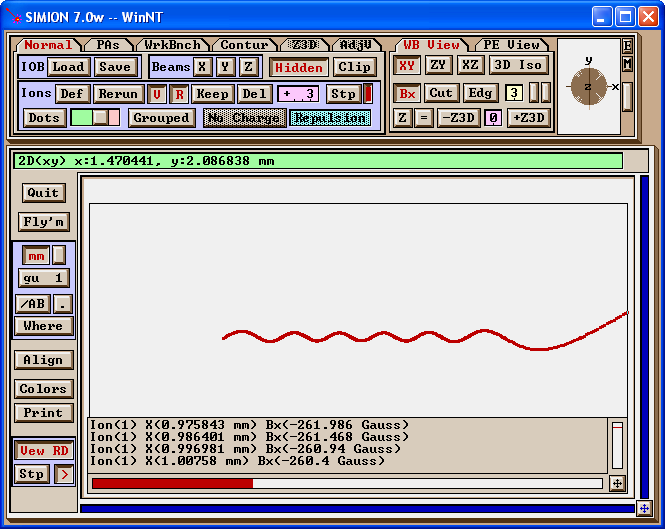
Figure: electron (1 eV at 10 degrees) flying though axial magnetic field generated by user program. Data recording displays Bx at each time step.
Caution: The simple formula above does not take into account radial field components and deviations off-axis. This means that the above code probably cannot be much relied upon to help with fringe-field effects. For example, a radial component can cause ion velocity changes in the axial direction even to the point of repelling an ion backward along the axis (see figure below). This effect is not demonstrated above. Unfortunately, the formulas for the general case are a bit more complicated (in fact, the above web page does not provide a full formula). Though an approximation might be done, it might be more worthwhile to use the other methods described in this article.
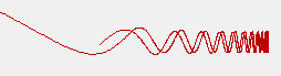
Figure: Low
energy particle repelled backward by an additional radial magnetic
field component.
The full SIMION project may be downloaded here: solenoidaxeq.zip .
Approach #1.2 - Interpolating the grid data
The second approach is to have the program read in the full CPO data file (of magnetic field vectors on a grid), and the user program would calculate the field vector at each point an ion moves to by performing an interpolation (e.g. a linear interpolation, though more complicated interpolations are possible as well) of values at the nearest surrounding grid points.
This program may be done in PRG code as described in the "Measured Magnetic Fields" section of the Advanced ASMS Course. PRG programs can be a bit difficult to write though for those who are not experienced with it, so one might alternately write an SL program as described in the complimentary article Exporting Electrostatic and Magnetic Field Data from SIMION (and Importing it too). Similar code for the solenoid example is omitted here due to the similarity.
Import Method #2: Constructing a PA file
Rather than writing a user program as in the first method, we might construct a regular potential array (PA) file. As discussed previously, this has some advantages such as not requiring user programming, and it permits potential and contours maps to be generated as usual in SIMION. Multiple approaches to this method are described below.
Approach #2.1: Converting the grid data to a PA file using the SL Tools
Here, we convert the CPO data file fairly directly into a SIMION PA file using the SL Tools "Text --> PA" function in the SIMION SL Toolkit. Overall, the process by the user is fairly simple. Internally, it is more complicated as discussed previously.
The first step is to transform the CPO output file ("solenoidtmpa.dat") into a PATXT file. The PATXT file generally holds the same information as a regular PA file but is in a human-readable ASCII text format with some additional smarts (e.g. you can specify magnetic fields rather than magnetic potentials). Fortunately, the PATXT file is also very similar in content and structure to the solenoidtmpa.dat file, differing mainly in that the PATXT file contains a "header" section describing for example, the size and symmetry of the PA and other things needed to construct the corresponding PA file from the PATXT file.
A portion of the solenoid.patxt file is shown below (the full file can be downloaded here: solenoid.patxt). This was created by manual text editing, and copying and pasting most of the solenoidtmpa.dat file into it. However, some transformation of the data is requirement, mainly to get the units right. Therefore, Excel was used (solenoid_field.csv) to translate the fields from Teslas to Gauss (multiply by 10000) and the coordinates from mm into grid units (currently, SL Tools requires that these coordinates be specified in grid units, but that might be improved).
# ASCII text representation of a SIMION PA file.
begin_potential_array
begin_header
    mode -1
    symmetry cylindrical
    max_voltage 10000
    nx 201
    ny 51
    nz 1
    mirror_x 0
    mirror_y 1
    mirror_z 0
    field_type magnetic
    ng 1
    fast_adjustable 0
    data_format field_y field_x y x
end_header
begin_points
0	14.445	0	0
0	14.992	0	1
0	15.568	0	2
0	16.174	0	3
0	16.811	0	4
0	17.482	0	5
Below shows using the SL Tools to transform solenoid.patxt into solenoid.pa.
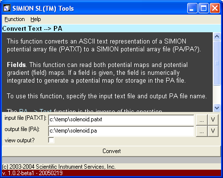
Figure: Converting solenoid.patxt to solenoid.pa using the SIMION SL Tools.
The generated PA file si shown below loaded into SIMION. Magnetic field contours have been drawn. Note how similar the contours appear to those of CPO (the same contour lines are used).
(One slight complication is that SIMION 7.0 requires at least one point on the PA to be a pole points for contours and potential maps to display. This fixed can be done in Modify.)
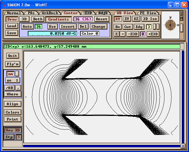
Figure: Magnetic field contours (0, 10, ... 350 Gauss) of PA in SIMION.
Note that the fields are only reasonable and accurate within certain well-defined areas. A PA defines scalar potentials, and in order for the scalar potential to even exist uniquely over some region of the field, the field must be conservative. Magnetic fields in particular are not always conservative--there is non-zero curl wherever there is current. In the case of the solenoid, there is current on the solenoid coil, so we can't compute potential there. We are safe if ions never fly within those problematic areas. (Some regions outside the non-conservative region are conservative but, for simplicity, are not calculated--this might be improved in the software.)
The axial field compared against the original data is shown below.
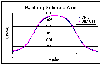
Figure: Axial magnetic field in SIMION compared to original CPO output.
To get a better idea of how reliable it is to convert this field to scalar magnetic potential (SIMION PA), the SL Tools was used to convert the potentials back to a field, and the that field was compared with the original field at every data point in the inside section of the solenoid:
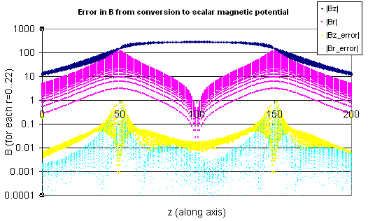
Figure: Error in B from conversion to scalar magnetic field for r=0..22 (center region of solenoid).
The relative error just inside the solenoid (r=0..22) is on average 0.06%, with the error increasing on approaching the solenoid coils (larger r), where there is a discontinutity. There's a spike of about 2% error on the boundary of the PA (z=0 and z=200), where the fields are not well defined. No particular attention was given to the accuracy and precision of the original field data.
Scalar magnetic potentials can also be shown. Normally, this data is less useful, but it provide some clues for a trick that will be used in the approaches discussed later.
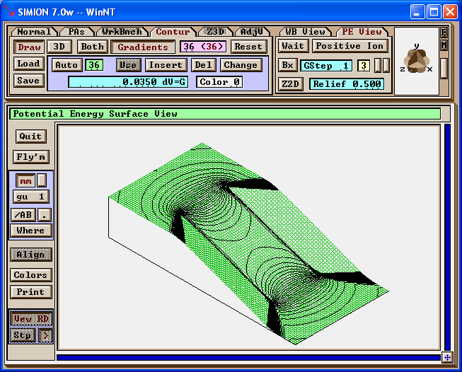
Figure: Magnetic potential map in SIMION, with magnetic field contours.
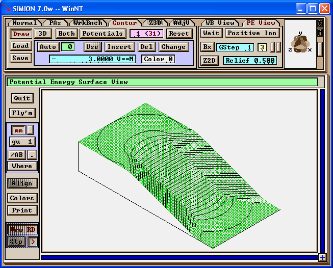
Figure: Magnetic potential map in SIMION, with scalar magnetic potential lines.
When viewing the above PA file in 3D, you will not see anything. The PA file is just an (invisible) field with has no real pole points. You would create actual poles by using the Find/Replace function in Modify (while preserve existing potentials). This would allow the object to have a visual appearance in 3D as shown below, and ions will splat against it.
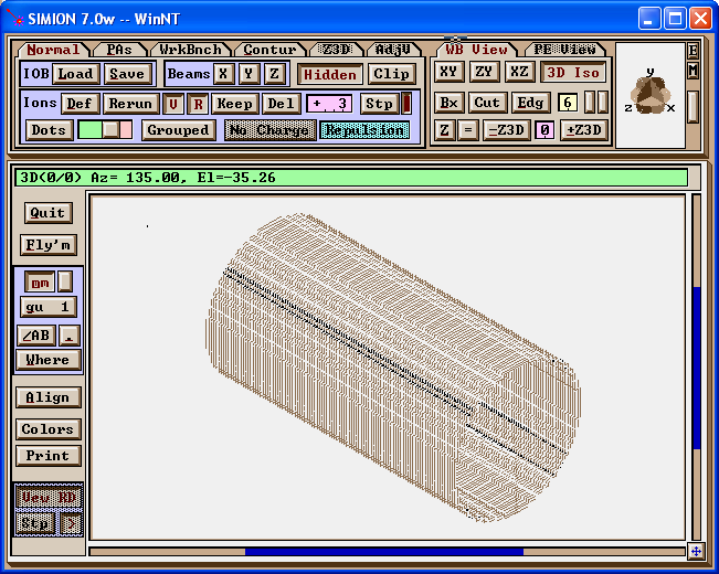
Figure: What the PA looks like in 3D if converting the singularities to pole points.
The potential array file may be downloaded here: solenoid.pa .
Approach #2.2: Constructing an approximate PA file manually from the grid data using Modify
The next approach does not use the SL Tools but instead uses a Modify trick in which we more manually input the potentials at only selected points on a boundary of interest, then use Refine to linearly interpolate to determine the full boundary, and use Refine again to solve for the interior points. The accuracy of this third method is likely somewhat less than the second method, assuming we are willing only to manually input a small selection of points. A form of this method was first noted in http://www.srv.net/~klack/forums.htm by David Dahl.
Let's have the solenoid exist on a (201 x 51 point) cylindrically symmetric grid of the same dimensions used in previous methods. For simplicity, we will be concerned with only the center section (the blue cylinder or radius 24 grid units shown below) that does not contain any poles or discontinuities. All area outside of this will be ignored.
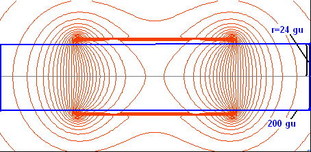
Figure: Blue box shows the boundary of the area we will be concerned with. We will define the potentials at selected points on the boundary.
We then define potentials (V) at selected points on the boundary (we will later have SIMION linearly interpolate the other boundary points). We first consider the upper boundary (which is identical to the lower boundary due to symmetry).
We know B along this boundary because CPO had calculated it, but we really instead need V when Modifying the PA. We can numerically compute V by applying the formula B = - grad V (assuming it holds), which involves solving the below line integral over B:
 = V(x_0,y_0,z_0) + \int_C \bf{B} \cdot d\bf{n}")
This can actually be much easier than it might first seem. Using the notation Vi,j and Bxi,j for the potentials and x component of the fields at the grid point (i,j) for i in 0..200, j in 0..50, we write:

Below are plots in Excel of Bx and V along the line r=24 (grid units).
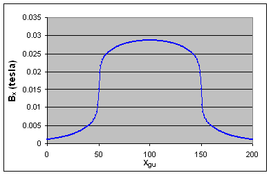
Figure: Bx at various points along the line y=24.
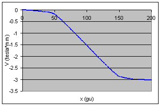
Figure: V at various points along the line y=24.
Notice that V can be approximated by a piece-wise linear function. It is especially linear inside the solenoid.
x	V
0	-0.0011168
25	-0.0453842
50	-0.1797209
150	-2.8656859
175	-2.9874107
200	-3.0301638
We will manually insert these points using Modify. In fact, we will rather draw vertical lines rather than points in order to utilize a trick in which Refine will linearly interpolate the potentials at the boundary points between the boundary points we define (this is a property of the Laplace equation). This is shown below.
Note below that we set the magnetic scaling factor (ng) to 10000, which is a factor that converts Teslas to Gauss; it may have been simpler to have just ensured that the fields we used above were in Gauss rather than Teslas. (Beware of units and double check that the field intensities and polarities you see in SIMION are reasonable!)

Figure: Creation of pole plates at x=0, 25, 50, 150, 175, and 200 gu.
We now Refine. The potential map of the result is shown below. Notice that the potentials on the boundaries are correctly linearly interpolated as desired. The non-boundary points are also linearly interpolated as a side-effect, but we can ignore this side-effect for now.
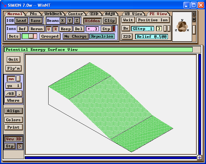
Figure: The potential map after refining.
Now, we use Find/Replace to change all pole points to non-pole points (without altering the potentials).
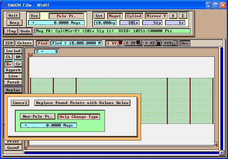
Figure: Change all pole points to non-pole points (while preserving potentials).
Next, we use Find/Replace to change points on the boundary from non-pole points to pole points (without altering the potentials).
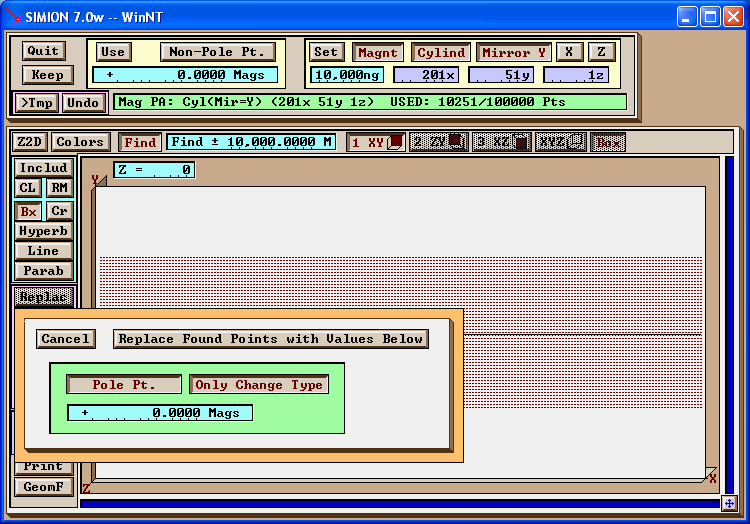
Figure: Change all (non-pole) points at y=24 to to pole points (while preserving potentials).
This completes the definition of the upper boundary. The result is shown below.
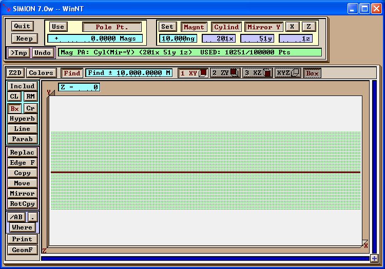
Figure: The result of the previous step. We now have a cylinder with the correct potentials along the surface.
We might define the potentials on the left and right boundaries as well. You can determine that these potentials are roughly uniform, and defining them have only minor effect in SIMION. For simplicity, we will ignore this boundary, but it may be more correct to define it (as typically required by the Laplace equation).
This PA can now be Refined to calculate the interior potentials. The result, with contours, is shown below. There is a slight but noticeable deviation in the contours compared to the previous results. This may be due to the choice of piece-wise linear approximation on the top/bottom boundaries (which could likely be improved) and the omission of the left/right boundaries. Also, improvement could be made by more accurately performing the integration or precisely scaling or aligning the potentials so that the fields in the very center of the solenoid are exact.
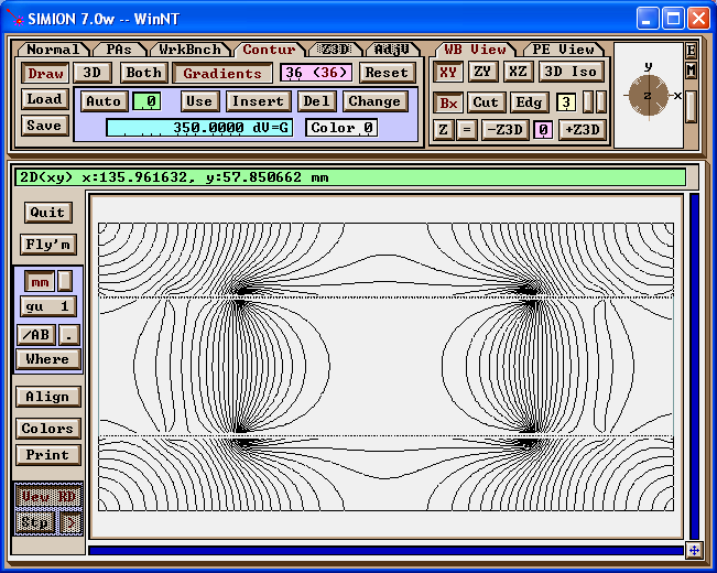
Figure: The result after refining.
Approach #2.3 - Constructing an approximate PA file with the SL Toolkit
A slight variation of the above Approach #2.2 is to use the SL Libraries in the SL Toolkit (rather than Modify/Refine) to set the boundary potentials, including possibly doing any interpolation between boundary points. This will make it easier to set the boundary potentials and possibly even all boundary points in a more automated manner than Modify. After the boundary is defined in the PA, use Refine.
Approach #2.4 - Constructing an approximate PA file entirely with Modify
Another modification of Approach #2.2 is to approximate the boundary points by inspection without even using an external program for the magnetic field calculation. This is a very accessible method and can be done rather quickly. At least it will provide an approximation that will be better than any uniform field assumption.
Conclusion
We examined the importation of a solenoid magnetic field into SIMION using both user programs and potentail array (PA) files. Various approaches were used including the calculation of the field in CPO, using a formula, and using approximations.
Comments and discussions may be placed in the forum.
Updates:
- Jan 2006 - added more complete error analysis for converting to scalar magnetic potential. (See chart "Error in B from conversion to scalar magnetic potential".)