Copyright © 2006-2008, 2000 Scientific Instrument Services, Inc.
SIMION® 8.0 User Manual.
SIMION® 8 (c) 2003-2008 Scientific Instrument Services, Inc. All Rights Reserved. SIMION 7 (c) 2005 Battelle Energy Alliance, LLC (BEA) on behalf of Idaho National Labs (INL). (c) 2000 Bechtel BWXT Idaho, LLC on behalf of Idaho National Labs (INL).
Printed in the United States of America.
Author: David Manura, Scientific Instrument Services, Inc. (SIMION 8, 2006-2008). David A. Dahl, Idaho National Laboratory (SIMION 7, 2000).
No part of this publication may be reproduced, stored in a retrieval system, or transmitted in any form or by any means--electronic, mechanical, photocopying, or otherwise—without the prior written permission of the publisher.
US GOVERNMENT. The United States Government is granted for itself and others acting on its behalf, a paid-up nonexclusive, irrevocable worldwide license in SIMION 7.0 to reproduce, prepare derivative works and perform publicly and display publicly. NEITHER THE U.S. NOR THE U.S. NOR THE U.S. DEPARTMENT OF ENERGY, NOR ANY OF THEIR EMPLOYEES, MAKES ANY WARRANTY, EXPRESS OR IMPLIED, OR ASSUMES ANY LEGAL LIABILITY OR RESPONSIBILITY FOR THE ACCURACY, COMPLETENESS, OR USEFULNESS OF ANY INFORMATION, APPARATUS, PRODUCT OR PROCESS DISCLOSED; OR REPRESENTS THAT ITS USE WOULD NOT INFRINGE PRIVATELY OWNED RIGHTS.
SIMION 7.0 resulted from work developed under Government Contract No. DE-AC07-99ID13727 at the Idaho National Laboratory (INL) and is subject to a Limited Government License. This work was supported by the U.S. Department of Energy INEEL (INL) internal research funds and by the Division of Chemical Sciences, Basic Energy Sciences, Office of Science, Department of Energy under contract 3ED102.
DISCLAIMER. These programs are provided "as is." It is the user's responsibility to determine the suitability of this material for any application. There is no expressed or implied warranty of any kind with regard to these programs nor the supplemental documentation. In no event shall the authors, Scientific Instrument Services, Inc., BEA, or the U.S. Government or any agency thereof be liable for incidental or consequential damages in connection with or arising out of the furnishing, performance or use of any of these programs.
- Introduction
- Basic Ion Optics Concepts
- The Potential Array
- The Role of the Subdirectory in SIMION Projects
- The SIMION Main Menu
- Building Your First Simulation from Scratch
- Creating a Project Directory
- Creating a New Potential Array in Memory
- Inserting Electrode Geometry
- Saving The Array as TEST.PA#
- Refining the Fast Adjust Potential Array
- Fast Adjusting the Voltages of the TEST.PA0 File
- Viewing the Potential Array
- Defining Some Ions to Fly
- Flying Ions
- Fast Adjusting Electrodes From Within View
- Saving Your Work
- Reloading Your Work
- Summary
Overview
This chapter summarizes some basic charged particle optics theory, introduces the fundamental SIMION concept of the potential array, and steps you through building your first simulation from scratch.
SIMION makes use of potential arrays that define the geometry of electrodes (or magnetic poles) as well as the potentials both on the electrodes and in the empty space between the electrodes. Typically, the potentials on the electrodes are defined by you, and SIMION solves for the potentials in the space between the electrodes (as well as the fields defined by the gradient of those potentials). The potentials between the electrodes are determined by solving the Laplace equation by finite difference methods (see Appendix H). In SIMION, this process is called refining the potential array. Refined potential arrays can then be positioned as potential array instances (3D virtual images) into an ion optics workbench volume. Ions can be flown within the workbench volume, with their trajectories calculated from the fields inside the potential array instances they fly through. This basic approach is the foundation for simulating a wide variety of charged particle optics systems.
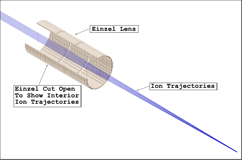
The illustration (Figure 2.1) shows ions flying through a simple einzel lens. The einzel lens has been cut open (a SIMION display trick) to show the ion trajectories within the einzel lens. The einzel lens has been created using a simple 2D cylindrical array. Cylindrical 2D arrays form volumes of revolution about their x-axis when refined and displayed ( function).
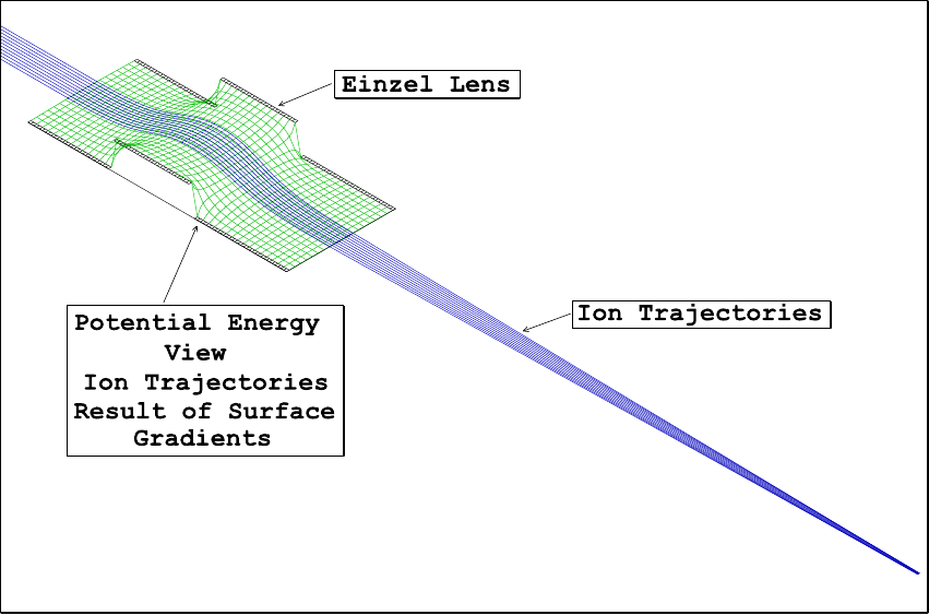
While this view of the ion trajectories is useful, it doesn't really explain why the ions are focusing. We can use SIMION's potential energy view (PE View) of the einzel lens to help us understand the electrostatic focusing process. Figure 2.2 shows a potential energy view of the einzel lens trajectories above. Note that the potential energy surface is much like the surface of a golf course. Since ions react in much the same way to potential energy surfaces as golf balls react to hills and valleys it is quite easy to see why ions have the trajectories they do in this einzel lens. SIMION's capabilities are designed to develop intuition and promote understanding.
Ion optics utilize the electrostatic and/or the magnetic forces on charged particles to modify ion trajectories. The following is a short (and simplified) summary of ion optics concepts. It is intended to summarize or introduce rather than educate. For further background, consult a introductory physics text on electromagnetics.
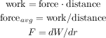
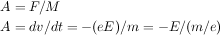
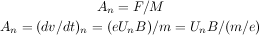
The movement of a particle (its acceleration) is defined by the force on it, as given by Newton's Second Law:
This force applied over a distance of movement is work (consuming energy):
The forces between charged particles are given by Coulomb's Law:
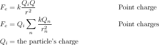
The electric field is the force per charge or (in terms of work) the change in work per charge (i.e. voltage) over distance:
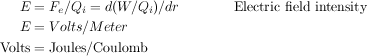
Conversely, we may think of the electric field as the cause of the force on a charged particle:

Putting this together, the acceleration on a particle (or it's trajectory) is determined by the electric field as such:
A magnetic field will also apply a force on a particle, but only if the particle is moving (non-zero velocity):
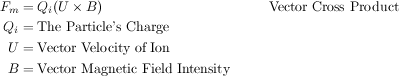
Magnetic force is always normal to both the B magnetic field vector and the U velocity component normal to the B magnetic field vector (following the right hand rule):

A simpler equation results from using only the vector velocity component normal to the magnetic field:

Putting this together, the acceleration of a particle (or it's trajectory) is determined by the magnetic field as such:
Note: Static magnetic fields change an ion's direction of motion but not its speed (kinetic energy).
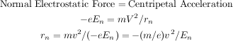
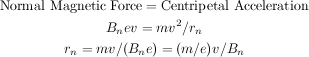
Refraction (bending of ion trajectories) results from electrostatic and/or magnetic forces normal (at 90 degrees) to the ion's velocity. We can determine the radius of this refraction.
The electrostatic radius of refraction is
The magnetic radius of refraction is
Interpretations of Radius of Refraction
The electrostatic radius of refraction is proportional to the ion's kinetic energy per unit charge. Thus all ions with the same starting location, direction, and kinetic energy per unit charge will have identical trajectories in electrostatic (only) fields. Trajectories are mass independent in electrostatic fields.
The magnetic radius of refraction is proportional to the ion's momentum per unit charge. Thus all ions with the same starting location, direction, and momentum per unit charge will have the identical trajectories in static magnetic (only) fields. Trajectories are mass dependent in static magnetic fields.
Because of the v verses v2 effects on the radius of refraction, magnetic ion lenses have superior refractive power at high ion velocities.
There are significant differences between light and ion optics:
Light optics make use of sharp transitions of light velocity (e.g. lens edges) to refract light. These are very sharp and well defined (by lens shape) transitions. The radius of refraction is infinite everywhere (straight lines) except at transition boundaries where it approaches zero (sharp bends).
Ion optics makes use of electric field intensity and charged particle motion in magnetic fields to refract ion trajectories. This is a distributed effect resulting in gradual changes in the radius of refraction. Desired electrostatic/magnetic field shapes are much harder to determine and create since they result from complex interactions of electrode/pole shapes, spacing, potentials and can be modified significantly by space charge.
Visible light varies in energy by less than a factor of two.
Ions can vary in initial relative energies (or momentum for magnetic) by orders of magnitude. This is why strong initial accelerations are often applied to ions to reduce the relative energy spread.
Light optics can be modeled using physical optics benches (interior beam shapes can be seen with smoke, screens, or sensors).
Ion optics hardware is generally internally inaccessible and must normally be evaluated via end to end measurements. Numerical simulation programs like SIMION allow the user to create a virtual ion optics bench and look inside much like physical light optics benches.
The electrostatic or magnetic field potential (e.g. Volts or Mags - SIMION's magnetic potentials) at any point within an electrostatic or static magnetic lens can be found by solving the Laplace equation with the electrodes (or poles) acting as boundary conditions. The Laplace equation assumes that there are no space charge effects and boundary conditions are sufficiently constrained.[1]
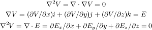
The Laplace equation constrains all electrostatic and static magnetic potential fields to conform to a zero charge volume density assumption (no space charge). This is the equation that SIMION uses for computing electrostatic and static magnetic potential fields.
Poisson's equation allows a non-zero charge volume density (space charge). When the density of ions becomes great enough (high beam currents) they will (by their presence) significantly distort the electrostatic potential fields. In these conditions, Poisson's equation should be used (instead of Laplace's) to estimate potential fields. SIMION does not support Poisson solutions to field equations. It does however employ charge repulsion methods that can estimate certain types of space charge and particle repulsion effects.
The Laplace equation really defines the electrostatic or static magnetic potential of any point in space in terms of the potentials of surrounding points. For example, in a 2-dimensional electrostatic field represented by a very fine mesh of points the Laplace equation is satisfied (to a good approximation) when the electrostatic potential of any point is estimated as the average of its four nearest neighbor points:

Physical models (as opposed to numerical models) have historically been used to solve many Laplace equation problems. These models have the advantage of giving physical insight into problems that can be difficult to understand.
Laplace equation solutions for electrostatic potential fields resemble surfaces of rubber-sheets stretched between electrodes where electrode height represents electrostatic potential. In fact, relatively flat rubber-sheet surfaces are good physical representations for electrostatic fields. Rubber-sheet models and marbles (for ions) have been used to model electrostatic fields (e.g. early vacuum tube design).
Resistance paper models have also been used. In this method electrodes of the designed shapes are pressed against paper having a uniform surface resistivity. Voltages are applied to the electrodes and electrostatic potential measurements are taken via a probe connected to a voltmeter. These measurements are then used to calculate ion trajectories.
Rubber-sheet models give the designer excellent insight into the behavior of ions in electrostatic fields. This is because we humans have each developed a certain physical intuition for the movement of balls on sloping surfaces (e.g. miniature golf). Note: SIMION's potential energy surfaces (Figure 2.2) use the rubber-sheet style of display to assist the user in developing intuition and understanding.
Unfortunately rubber-sheet models are difficult to build. Moreover, they are limited in their modeling accuracy because forces are proportional to the sine of the slope (e.g. g dh/dr) rather than the tangent of the slope (e.g. dV/dx) needed in electrostatic ion optics.
SIMION utilizes potential arrays to define electrostatic and magnetic fields. A potential array can be either electrostatic or magnetic but not both. If you require both electrostatic and magnetic fields in the same volume, array instances of electrostatic and magnetic arrays must be superimposed in the workbench.
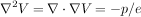
A potential array is an array of points organized so the points form equally-spaced square (2D) or cubic (3D) grids. Equally-spaced means that all points are equal distances from their nearest neighbor points. Figure 2.3 shows a function view of a 51 by 51 2D potential array.
All points have a potential (e.g. voltage) and a type (e.g. electrode or non-electrode). Certain points are flagged as electrode or pole points. Points of type electrode/pole create the boundary conditions for the array. Groups of electrode points create the electrode and pole shapes (the finer the grid the smoother the shapes). Non-electrode and non-pole points within the array represent points outside electrodes and poles. We need to solve the Laplace equation to obtain the potentials of these points (the non-electrode and non-pole points.)
Potential arrays are dimensioned by the number of points in each dimension (x, y, and z). Therefore an array of nx = 51 would have 51 points in the positive x direction. All arrays have their lower left corner at the origin (xmin = ymin = zmin = 0). Thus if nx equals 51, xmin equals 0 and xmax equals 50 (a width in x of 50 grid units).
Note
If a PA contains 51 grid points along one dimension, the points will be at integer positions 0 to 50 grid units, and the PA will have a physical width of 50 grid units (not 51).
All 2D arrays have nz = 1 (zmin = zmax = 0). Thus 2D arrays are always located on the z = 0 xy-plane.
Arrays can use a lot of memory. A 100x by 100y by 100z 3D potential array requires one million points. Each point requires 10 bytes of RAM. Thus 10 megabytes of RAM are required for each million array points.
Note
Each point requires 10 bytes of RAM. SIMION 8 supports up to about 200 million points (under 2 GB) in a PA.
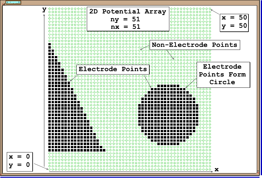
Two potential array symmetries are supported: Planar (2D and 3D arrays) and cylindrical (2D arrays only). When SIMION refines (solves the Laplace equation) or projects an array instance (3D image) of an array into its ion optics workbench volume, it uses the array's symmetry. If the 2D array has a cylindrical symmetry it will be projected to create a volume of revolution about its x-axis. Figure 2.4 (top-left) shows an isometric 3D view of the array in Figure 2.3 assuming it has cylindrical symmetry. Note: The cylindrical 2D array is visualized as if it were 3D planar to take advantage of fast planar visualization methods. However, apertures are really round (despite how they appear) and the cylindrical symmetry is fully retained for ion trajectory calculations.
In contrast, Figure 2.4 (top-right) shows an isometric 3D view of the array in Figure 2.3 assuming it has 2D planar symmetry. Note that 2D planar symmetry assumes that the array itself is only one layer of an infinite number of layers in z (for refining purposes). When SIMION projects a 2D planar array as an array instance within the workbench volume it assumes a z depth of +/- nz (grid units). You may edit the array instance definition to increase this z depth. This option allows a 2D planar array to be used to represent the interior (symmetrical) portions of objects like quadrupole rods (saves array space).
Many electrode designs have a natural mirrored symmetry. Designs that mirror in y have a mirror image of the electrode/poles in the negative y. SIMION supports three mirroring symmetries: x, y, and z. Mirroring allows you to use a smaller array to model a larger area (or volume) when conditions permit. For example: A 3D planar array can be mirrored in x, y, and/or z. If the design symmetries permit, this would allow the modeling of a 3D volume with one eighth the number of points required if no mirroring were utilized. SIMION takes mirroring into account when refining arrays and projecting their instances into the workbench volume.
X mirroring is allowed for all 2D and 3D arrays. Y mirroring is required of 2D cylindrical and allowed in 2D and 3D planar arrays. Z mirroring is only allowed in 3D planar arrays.
Figure 2.4 (bottom) shows mirroring enabled on both the cylindrical (bottom-left) and planar (bottom-right) geometries discussed previously.
SIMION uses the same finite difference methods for refining either electrostatic or magnetic potential arrays. However, the definitions for potentials and gradients used are different and it is important that you understand these differences.
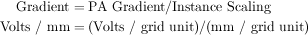
Potentials in electrostatic arrays are always in volts. SIMION uses the refined array potentials to determine field gradients (voltage gradients). Electrostatic field gradients are always in volts/mm. When an array instance of a potential array is projected into the workbench volume, it is scaled by a user specified number of millimeters per grid unit (or defaulted to 1 mm/grid unit). So although electrostatic gradients start out as volts/grid unit they are divided by the instance scaling factor to obtain volts/mm:
Thus array instance scaling can have a dramatic impact on electrostatic gradients and therefore ion accelerations.
SIMION is not a magnetic circuit program. You have to supply the magnetic potentials for it to refine. Unlike electrostatics, in magnetics we normally think of and measure gradients or more precisely flux (gauss) as opposed to potentials. This presents a problem because SIMION needs scalar magnetic potentials to refine.
In order to deal with this dilemma SIMION defines magnetic potentials in Mags. Mags are defined to be gauss times grid units. Thus the gradient of magnetic potential is simply gauss. Note: Mags are gauss times grid units instead of gauss times millimeters. If Mags were gauss times millimeters then instance scaling would confound us further. With this approach, magnetic fields remain the same whether the array is scaled to be a certain size or 10 times as large in the workbench volume. Thus instance scaling has no impact on the magnetic fields (flux in gauss) produced by magnetic potential arrays.
SIMION also makes use of a magnetic scaling factor ng as a property of magnetic potential arrays. The ng scaling factor has been provided to further simplify your life. It would often be very nice for Mags to be directly related to gauss. Let's say we have a simple two pole magnet. We would like to set one pole to 1000 Mags and the other to Zero Mags and have the field in between be approximately 1000 gauss. If the two poles are separated by let's say a 60 grid unit pole gap we would specify the value of 60 for ng to automatically scale the Mags potentials roughly into gauss.
Note: The B field vector always points from greater magnetic potential (e.g. 1000 Mags) toward lesser magnetic potential (e.g. 0 Mags).
Beware! Magnetic potentials are not as simple as electrostatic potentials, and some magnetic fields cannot be expressed as scalar potentials but rather as vectors. While we can safely assume that all points of an electrode have the same electrostatic potential (e.g. volts), it is dangerous to assume that the same is generally true for magnetic poles. Magnetic poles do not as a rule have totally uniform magnetic potentials across their surfaces (permeability not being infinite). Thus you must allow for this fact if the effects could be significant enough to impact your results. Remember: User beware. [2]
User defined potential arrays come in two classes the
basic potential array (.PA
file extension) and the fast adjust definition array
(.PA# file extension).
The basic potential array has its electrode/pole potentials
defined as described above. These arrays are then processed by the
function to solve for the non-electrode and non-pole
potentials. The basic array is always saved with a .PA file
extension. An array's file extension is important
because SIMION assumes that all arrays with a .PA file
extension are basic potential arrays for refining, adjusting, and
viewing purposes.
The fast adjust definition array is much like the basic
potential array except the electrode potentials are not explicitly
defined but rather are indices to potentials that are defined later
(after refining). Here, the Laplace equation is solved
independently for each electrode. Using the additive
property of the Laplace equation, these independent solution can then
be linearly combined for any desired combination of electrode
potentials. In this way, you may adjust the potentials on the
electrodes quickly--hence the name fast adjust--without the
relatively slow step of re-refining. This even makes practical things
like simulations of quadrupole rod oscillations in the megahertz
range. All fast adjust definition arrays must be explicitly saved
with a .PA# file extension so that SIMION will recognize and
process them properly.
We often need to change the electrode/pole potentials of an already refined array to tune a lens or adjust a magnet's field. SIMION supports three different strategies:
The first strategy is the brute force approach:
Use the function to change the potentials of the points of one or more electrodes or poles in the basic potential array (
.PA).The use the function to re-refine the basic potential array (
.PA) to obtain the resulting potentials of the non-electrode or non-pole points.
This is the - cycle of array potential adjustment. It is time consuming and invites errors (e.g. accidentally not changing the potentials of all the points defining an electrode or pole).
SIMION also supports proportional re-scaling of
all basic potential array (.PA arrays)
potentials. This is useful in those cases when the potentials of all
electrodes or poles can be changed proportionally to obtain the
desired result. This approach works with any basic potential
array (with .PA file extension) that has already been
refined:
Use the function to change the potential of the highest absolute potential electrode or pole in the potential array (displayed as electrode 0). The only illegal proportional scaling potential is 0, because a re-scaling potential of zero would cause all the potentials of all points in the array to be zeroed, and thus the refined field solutions would be lost (irreversible scaling).
SIMION will automatically scale the potentials of all array points (electrode/pole and non) by the same proportion that you changed the potential of the highest potential electrode or pole.
This can be quite useful for a magnetic potential array with two poles and a gap. Proportional scaling provides a quick way to adjust the magnetic field. It even supports proportional scaling of non-uniform potentials on the pole surfaces (fringe field effects). This is a clever trick only if you can justify that these non-uniform pole surface potentials actually would scale proportionally in your problem.
The third approach, offered by fast adjust definition arrays
(.PA# files) makes use of the additive solution property of
the Laplace equation. This involves creating a separate array for
each electrode we desire to adjust, setting the points of the desired
electrode/pole to a fixed potential, and setting all other
electrode/pole points to zero. Each of these separate electrode
arrays is then refined, and each refined electrode solution array is
then saved to disk.
Composite fields are obtained by scaling each electrode's solution array to its desired voltage and adding the individual field contributions of the various adjustable electrodes together to obtain the desired result. This is all quite fast (avoids re-refining) if you can keep track of all the book-work. Fortunately, SIMION is designed to do all the hard work for you!
Use the function to define the geometry of your electrodes. All points of the first adjustable electrode (pole) must be set to exactly 1 volt (Mag). Likewise, all points of the second must be set to 2, and so on. Adjustable electrode/pole potentials must not be skipped (e.g. 1,2,4,5).[3] Up to 127 adjustable electrodes can be defined in this manner within a potential array. Non-adjustable electrodes or poles may also be defined provided they do not have the exact potentials from 1 to 127 (e.g. 10.0001 volts is OK).
Save this potential array to disk with a
.PA#file extension to signal to SIMION that this is a fast adjust definition file (e.g. save asTEST.PA#).Refine the
.PA#file. SIMION will recognize that this is a fast adjust definition file, examine it, create each required electrode solution array, refine them, and save them to your disk automatically.SIMION creates individual fast adjust electrode solution arrays for each adjustable electrode and refines them automatically. These have the extensions
.PA1 - .PA127[4] (Electrode one is stored in a.PA1file, e.g.TEST.PA1).If non-zero potential non-fast adjustable electrode points are found (e.g. 10.56 volts) in the
.PA#file, SIMION automatically creates and refines a fast scaling solution file for these points called.PA_. This allows you to proportionally re-scale these electrode points as electrode 0 in a manner similar to that described above, except that a 0 proportional scaling potential is allowed because the solution is preserved in the.PA_solution file.[5]Finally, SIMION creates a base solution array
.PA0(e.g.TEST.PA0). This array initially contains the potentials of all non-fast adjustable electrodes/poles, but these potentials can be adjusted later. The.PA0array is called the fast adjust array because this is the final array you actually fast adjust (and fly ions through).Use the function on the
.PA0file to set potentials. Fast adjust electrodes will be numbered from 1-127 and the fast proportional scaling electrode points (if a.PA_file was automatically created) will be changed via electrode 0. If you try to fast adjust a.PA#file SIMION will automatically load its.PA0file for adjustment. If you want to save the current potential settings of a.PA0file between SIMION sessions, simply save the.PA0file to disk.
The function is accessible from the Main Menu Screen or from within the function (even while ions are flying).
SIMION maintains a working copy of each active potential array (up to 200) in memory (RAM). When you change something in a potential array you are only changing the in-memory copy. Likewise when you fly ions through instances of potential arrays in the workbench you are using the in-memory copies of the potential arrays.
User defined potential arrays are normally saved as
.PA or .PA# (extension) files in your
project directory. When you create a new potential array only
the in-memory copy is created. It is your responsibility to save any
new or changed potential arrays to your project directory as required.
Saving potential arrays preserves your work between
sessions.
Potential arrays can use up a lot of memory. Each point of a potential array requires 10 bytes of RAM storage. Thus a 100 x by 100 y by 100 z 3D array has 1,000,000 points and requires 10 megabytes of RAM. SIMION allocates memory only once for each PA memory region it creates. Once the PA memory has been allocated it is not returned or changed until the button is used to remove all memory allocated PAs (de-fragment the heap). This is done to prevent heap fragmentation lockups due to the large size of typical potential arrays.
SIMION requires that all files relating to a
project (e.g. *.PA, *.IOB, *.FLY2, and
etc.) be contained in the same subdirectory of your hard
disk. This is useful because it keeps things together and in so
doing forces a touch of organization that many of us need so badly.
Note: There can be more than one project in a subdirectory. However,
this can often create a lot of clutter.
Important
SIMION requires that all files relating to a project be contained in the same folder. Ignore this at your peril!
Each of the demos provided with SIMION is in its own directory
below C:\Program Files\SIMION-8.0\examples. These demos
help show how various projects might be approached.
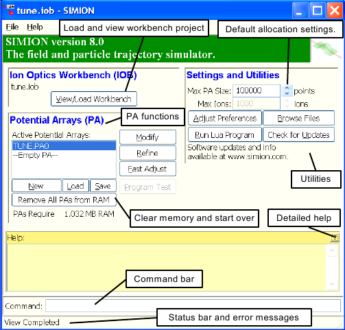
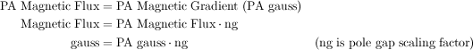
Figure 2.5 shows the SIMION Main Menu Screen.
This is the first screen you will see in SIMION. It serves as the
point of departure for all SIMION adventures. The buttons in the center
allow you to access the various primary functions
(e.g. ). Notice that the first letter in
each button's label is underlined. This means that you
can access a particular button by either clicking on it
with the mouse or by entering the underlined key from
the keyboard (e.g. m for ).
The list on the left contains all the potential arrays currently
in RAM (in this case, one: MIRROR.PA). Other
objects (buttons and etc.) are used to display and control or
modify the potential array (more of this later).
Note
The button can be used to check for free software updates from simion.com.
Note that 8.0.x or additional updates to the SIMION software may be available (possibly monthly). The button will open a page on the simion.com web site to allow you to download these updates.
The button allows you to adjust various SIMION and GUI characteristics. Clicking the button brings up a screen that allows you to change colors, sounds, and other options. If you haven't explored , do it now. Descriptions of all options can be found in the GUI discussion in Appendix C.
The Main Menu Screen (Figure 2.5) contains a window with a list of each currently allocated PA memory region and the name of the potential arrays in each (long file names are supported - however a long file name may be displayed truncated to fit the width). One of these will be selected as the currently active potential array. This is the array that will be acted upon by functions like: , , , , , etc.
A particular potential array is selected by clicking (depressing) its button.
The last button in the list is always marked empty PA. This empty PA is available for allocating memory for a new potential array. Up to 200 potential arrays can be loaded in RAM at one time.
The following material is an illustrated step-by-step example of how to create an electrostatic potential array and use it to fly ions. It is recommended that you use SIMION to follow along with the example below. The best way to learn SIMION is to use it.
To begin, start SIMION.
The first step in starting any new SIMION project is to create a project directory to hold all the files you'll create. Remember, SIMION expects that all project files reside in the same directory. You ignore this rule at your peril!
Let's create a new directory called basic that is
directly below the c:\Program Files\SIMION-8.0\mystuff
directory (or anywhere else you may like). On convenient way to
this is shown (Figure 2.6):
Click the button.
In the file browser dialog box, navigate to the
c:\Program Files\SIMION-8.0\mystuffdirectory (or any other folder of your choice) if you are not already there.Click the button for creating a new folder (Figure 2.6) and type
basicas the file name.Then press to exit from the function.
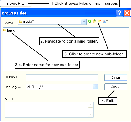
The next step is to create a new potential array in memory (Chapter 4). Use the following steps for this example (Figure 2.7):
If the list of potential arrays on the main screen is not empty (it should be), click the button.
Click the button to access the Potential Array Creation Screen.
Adjust the x dimension panel to 51 and the y dimension panel to 25. We will use the defaults for all the other array parameters.
Click to create a new potential array.
For this exercise, we are going to make a fast adjust
definition array (.PA#) of a simple three element lens. It
is a useful example because fast adjustable arrays are the most
commonly created array type. The choice of a simple three element
lens provides something to play with that will give you insight into
how electrostatic ion optics really work.
The function will be used to define the electrode geometry. also can be used to change array dimensions, symmetry, mirroring as well as edit the geometry definitions of any existing potential array (Chapter 5).
We are going to create three adjustable electrodes. Electrode number one will be a circular plate on the left edge of the array. Electrode number two will be a disk with a hole in it in the center of the array (remember this is a 2D cylindrical array). Electrode number three will be a circular plate on the right edge of the array.
Electrodes will be at least two array points thick so that SIMION will treat them as solid objects rather than as grids when flying ions (Chapter 5).
Array points defining electrode number one will be 1.0 volt, those for electrode two will be 2.0 volts, and those for electrode three will be 3.0 volts. This is required for SIMION to recognize these points as adjustable electrode points.
Click the button on the Main Menu Screen to access the function. You should now be looking at the Screen (Figure 2.8). Each electrode is defined by setting its point type (e.g. electrode) and voltage, marking its area of points, and then clicking the button to replace the marked points with the defined values. The followings steps should be used:
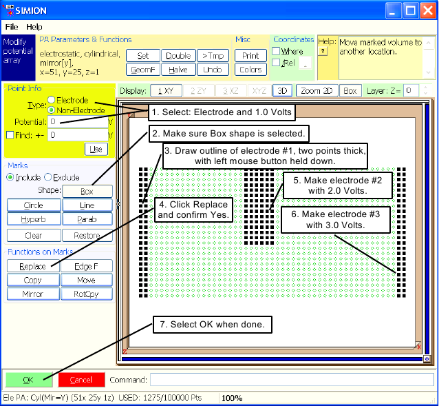
For electrode number one, make sure point type is selected and set the Potential panel to 1.0 volt.
Check to see that the (box) button is depressed. It selects box area marking.
Now move your cursor to the upper left corner point of the array. Hold down the left mouse button, and drag the cursor (keeping the left mouse button depressed) to the bottom of the array one point to the right (to mark an area two points thick). Now release the left mouse button and the area is marked. If you make a mistake marking, just re-enter the correct mark.
Click the button and click the button to replace the points in the marked area with 1 volt electrode points. If the wrong points are marked, you can erase them by changing the point definition to Non-Electrode of 0.0 volts, marking the error's area, and doing to replace the marked points with non-electrode 0.0 volt points.
Change the Potential panel to 2.0 volts and insert electrode number two (as in Figure 2.8) in the same manner as electrode one.
Change the Potential panel to 3.0 volts and insert electrode number three on the right edge (as in Figure 2.8) in the same manner as electrode one.
When you're done creating the electrode definitions, click the button to exit and keep the array changes (in-memory copy).
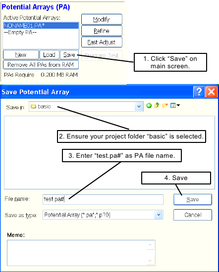
At this point the only copy of this array is the in-memory copy.
SIMION has assigned it a temporary name of NONAME01.PA and
has a asterick (*) after it to indicate that it is not saved
(and possibly also an exclamation (!) symbol to indicate
unrefined). We next need to save this file as test.pa# in
the basic directory. The .PA# file extension
tells SIMION that this is a fast adjust definition file
(important). Use the following steps to save the array
(Figure 2.9):
Click the button on the Main Menu Screen.
Make sure the current directory is
basic(if not, nativate to it)Enter
test.pa#in the File Name Notice there is also a Memo field. You have the option of entering a short description of this file (memo) for future reference, or you may skip this.Press Enter. The Main Menu Screen returns.
The next task is to refine the potential array (solve
for the electrostatic fields). When you refine a .PA#
potential array SIMION doesn't actually refine the .PA#
array itself. It uses the .PA# array as a definition for
the collection of arrays (one per each adjustable electrode
plus one for the combined solution) that actually
creates, refines, and saves in the current directory (basic).
Use the follow steps to refine the array
(Figure 2.10):
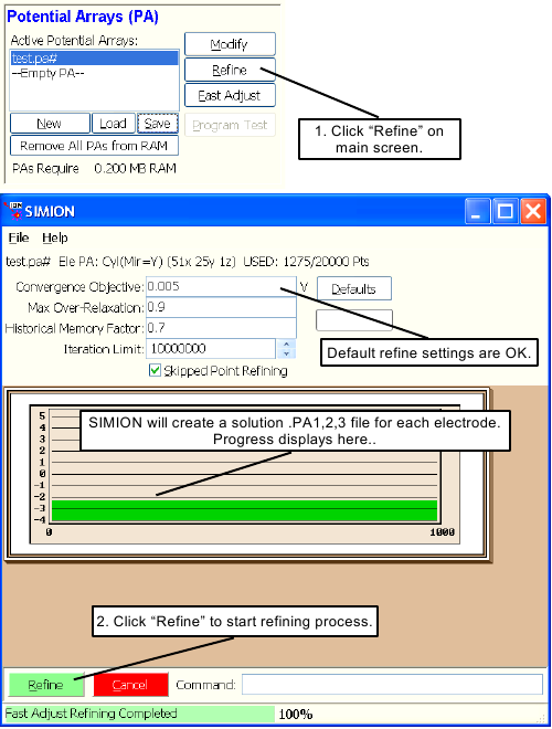
Check to see that
TEST.PA#is the currently selected array on the Main Menu Screen). Click the button. You should now be looking at the Screen (Figure 2.10).Click the button to start the refining process.
SIMION will scan the array, determine the number of
adjustable electrodes, create each of the four required arrays
(.PA0, .PA1, .PA2, .PA3),
refine each array and save them in the basic
directory.
When all this is completed, you will be returned to the Main
Menu Screen. You can verify that these four fast adjust support files
have been created by clicking on the button to
look at the contents of basic
(Figure 2.11).
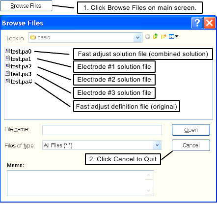
The .PA1, .PA2, and .PA3 files
contain the respective solutions for each of the adjustable
electrodes. If there had been one or more non-zero non-fast
adjustable electrode points (e.g. one with a non-integer
voltage such as 5.6 volts), SIMION would have automatically created a
.PA_ fast scaling solution file as well for those voltages.
The .PA0 file is the final solution array you will fast adjust
and fly ions through.
In the dialog box, click the Cancel button or hit the Esc key to return to the Main Menu Screen.
The actual fast adjust file is the TEST.PA0
file (the fast adjust definition file was the
TEST.PA# file). This file contains the final solution,
accounting for all electrodes adjusted to their final voltages (in
this case, the final voltages will actually be 1000V, 1000V, and 0V,
not 1V, 2V, and 3V).
Initially, all adjustable electrode voltages are set to zero in
the .PA0 file.
The TEST.PA0 file is the file we must actually fast
adjust. We could load it in place of the TEST.PA# file by
clicking the button and selecting the
TEST.PA0 file button to load the file. However, the
function will do this automatically anyway.
When clicking the button (assuming that
the TEST.PA# file is currently selected), SIMION
looks at the file, sees it is a .PA# file, and
automatically loads the .PA0 file in its place.
SIMION then allows you to fast adjust it
(Figure 2.12).
We want to set electrode number one to 1,000 volts, electrode number two to 1,000 volts, and electrode number three to 0 volts (its current value). Use the following steps:
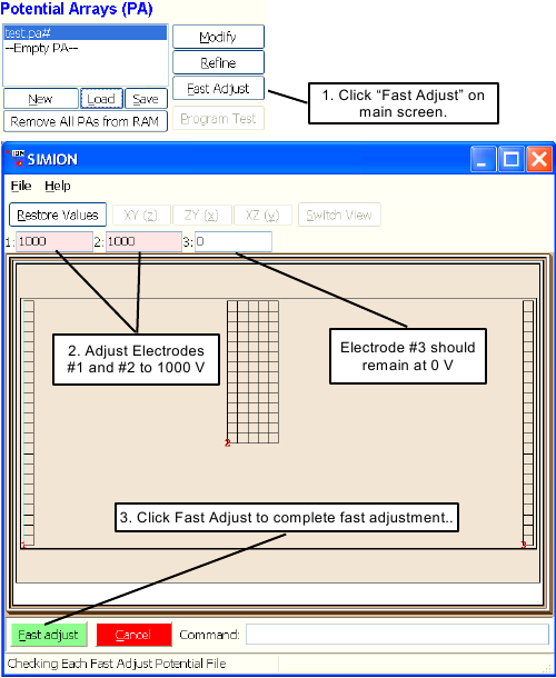
With the
TEST.PA#file selected, click the button. SIMION automatically loads theTEST.PA0file in its place and displays the screen.Adjust electrode number one's voltage to 1,000 volts using its panel object and adjust electrode number two's voltage to 1,000 volts also. Note: SIMION automatically draws a red line connecting an electrode's voltage control panel with one of its electrode points when the cursor is in the panel object so you can see which electrode the electrode numbers refer to.
Click the button and the array is fast adjusted.
Note: SIMION fast adjusts the in-memory copy of
the .PA0 file. If you want to retain these values between
sessions you should save the updated in-memory copy back to disk.
For example: Click the button, hit the Enter key
(to save), click to replace.
To view the TEST.PA0 potential array, make sure its
selected in the potential array list on the main screen and click the
button. Your screen should look like
Figure 2.13.
You can click the , , and buttons to see other standard views. Adjust the Display Quality panel from 0 (lowest quality) to 9 (highest quality) in view to see what it does. Also use the Orientation Sphere object to change views (point the cursor to it and drag the sphere about with either mouse button depressed). There are twelve 2D and eight 3D standard views. See if you can use the Orientation Sphere to see them. When you're through exploring, click the button to return to your starting view.
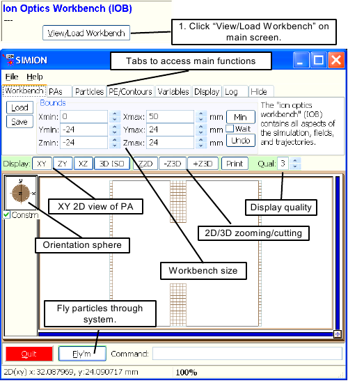
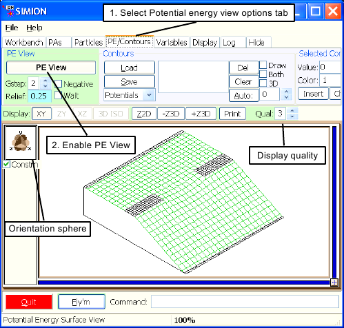
Figure 2.14 shows a potential energy view of the potential array. To duplicate this view, click the button (or make sure it is depressed) and then click the PE/Contours tab and press down the button to switch to a potential energy view. The PE view is also affected by the Display Quality and Orientation Sphere controls.
The next task is to define some particles to fly (Figure 2.15).
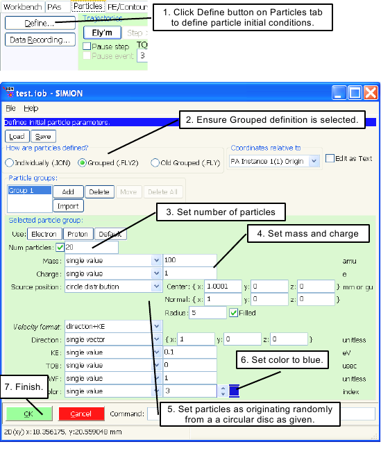
Select the Particles tab and click the button. You should now be looking at the Particle Definition Screen.
Make sure that Grouped is selected. SIMION allows us to define ions by two methods: Individually or by Grouped. For this example we will define ions Grouped.
Set the number of particles in group 1 to 20 using the Num particles panel.
Set the mass and charge to 100 u and +1 e respectively using the Mass and Charge panels..
Set Source Position to circle distribution, change its x coordinate of the Center to 1.0001 (to start just to the right of electrode number one), change the Radius of the circle to 5, and check the Filled box. This causes the ions to eminate from the surface a disc (filled circle).
Set the color of the ions to blue (3) using the Color panel.
Now click to keep the definitions and return to the Screen.
Click the button to fly the defined ions. Your screen should be something like Figure 2.16 if you're still in a PE View.
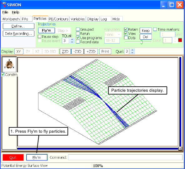
You can fly the ions together by selecting the Grouped check box before you click . Further, you can keep the ions flying by selecting the check box too. It gives a movie effect (click again or hit the Esc key to stop). Trajectory computations will speed up if you change the Trajectory Computational Quality panel from 3 (its default) to 0 (for a simple simulation like this, SIMION may calculate these too quickly already to notice a difference). There are all sorts of things to learn and try for yourself!
SIMION allows you to fast adjust electrodes from within the
function. To accomplish, click the PAs tab,
select the test.pa0 in the PA Instances list (it
is already selected since there is only one to select in this
example), and click the button.
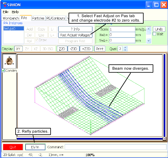
For this example adjust the voltage of electrode number two to zero volts and fast adjust it. Now click the button. Notice the shape of the potential energy surface has changed dramatically. The ions diverge rather than focus (Figure 2.17).
Let's assume we want to adjust the voltages so that the ions just focus when they hit electrode number three. The first step is to enable the Rerun and Grouped check boxes (on the Particles tab). Now click the button. Notice that the ions keep flying like in a movie. Under the PAs tab click the (Voltages) button to enter the Fast Adjust screen. Change electrode number two to 900 volts and . Check the focus. If it's not quite right click the button and try again. This is known as interactive tuning.
It is important that you save your work. This allows you to
quickly resume your efforts in a subsequent SIMION session. The
following material shows you how to save your .IOB file
(ion optics workbench definition file) as well as saving an
auto-loading .FLY2 (ion group definition
file).
An ion optics workbench file (.IOB)
retains the current workbench definitions. These include the
dimensions of the workspace, the names of the potential arrays used,
their adjustable potentials, and the array instance definitions of how
these potential arrays are to be projected into the defined
workspace.
To save the current workbench definition (including the
voltages used in all instances), click the Workbench tab.
If ions are currently flying from the above adventure, click the
button (or hit the Esc key)
to stop the flight. Now click the button on the
Workbench tab, enter the word test for a file name
and hit the Enter key. SIMION will automatically append the
.IOB extension to the file, and save your current workbench
definitions as test.iob in the basic directory
(assuming it's the current directory).
You can save more than one .IOB file. Let's say you
wanted to save an .IOB with different voltage settings. You
would adjust the electrodes to the desired voltages and then
save an additional .IOB file (perhaps
test1.iob) in the same manner you saved test.iob
above.
This example brings up the issue of file memos. If you choose
to use names like test.iob and test1.iob you will
probably not know which one to choose a month (or day) from
now. Although SIMION now supports the use of long file names
(e.g. My First Try at SIMION.iob), you may want to
consider attaching a file memo to each file when it is saved to
describe its features or other details.
You can verify that the file has your memo by selecting a file in or any file dialog box. When a file is selecetd, the memo will display automatically.
When you save an .IOB file SIMION will always
ask you if you want to save an auto-loading ion definition file too
(.FLY2 or .ION depending on the ions
currently defined). If you click , SIMION will save
the appropriate ion definition file with the name of the
.IOB file and proper ion definition file extension
(e.g. test.fly2 for the above example). This ion
definition file will automatically be loaded whenever its associated
.IOB file is loaded (handy).
You also have the option of saving ion definitions to files of
your choice. In this case, click the button on the
Particles tab. Now click the button, enter
the words First Ion Definitions for a file name and hit the
Enter key. SIMION will automatically append the
.fly2 extension to the file, and save the current ion group
definitions as First Ion Definitions.fly2 in the
basic directory (assuming it's the current
directory).
Let's pretend that this is a new SIMION session and that we want to reload that landmark simulation that we performed above. Click the button and button to exit from back to the Main Menu Screen. Now click the button and to return all of PA memory to the available memory heap. SIMION now has no files loaded.
Click the button. SIMION doesn't
have a potential array to view (the Empty PA
is selected in the list of potential arrays), so it
automatically opens the file selection dialog box and prompts you to
select an .IOB file. Select the test.iob file
(saved above). SIMION will load the .IOB file and
all the potential arrays it references.
SIMION will now check for auto-loading files. In this case it
will find a file called test.fly2 (assuming you said
to saving an auto-loading ion definition file when the
test.iob> was saved). This file will be automatically
loaded.
SIMION also can save and auto-load other files. These include
.ION (ion by ion definitions), .REC
(data recording), and .KEPT_TRAJ (kept ion
trajectory files). These features are discussed in
Chapter 7.
We have covered a lot of ground in this chapter. While this information should serve to get you started with SIMION, there is a whole lot more to learn. You have the option of either using the F1 (help) key to crash, burn, and learn; or you can keep on reading.
It is recommended that you read a bit and use SIMION a bit. This is probably the quickest way to learn how to use SIMION effectively. As you learn, try to use SIMION for some real problems, but be careful not to be too ambitious with what you tackle until you have learned the techniques to attack it properly.
The Adventure Continues . . .
[1] Sufficient conditions can be obtained under so-called Dirichlet and/or Neumann boundary conditions. For example, if the voltages on some closed boundary surface are defined (Dirichlet conditions), as often done in SIMION, then the Laplace uniquely determines ths potentials at all points inside the surface; if not, beware. See also SIMION Info: First Uniqueness Theorem. http://www.simion.com/info/First_Uniqueness_Theorem .
[2] Some additional notes on the issues of simulating magnetic fields in SIMION are at SIMION Info: Magnets http://www.simion.com/info/Magnets .
[3] This restriction was removed in 8.0.4: http://simion.com/issue/414
[4] Note to SIMION 7
users: SIMION 7 used letters in the extensions for adjustable
electrode 10 and beyond, i.e. .PAA - PAU, while SIMION 8
uses only numbers to more cleanly support a larger number of
adjustable electrodes without confusion. This is one of the few
possible file format incompatibilities between SIMION 7 and 8, but it
may be easily resolved by rerefining in SIMION 8.
[5] 8.0.3 allows multiple fast scaling solutions, which are useful for ion funnels and resistor chains. See http://simion.com/issue/172