Collision Model HS1
This SIMION user program implements a rather complete hard-sphere collision model. Collision models are useful for simulating non-vacuum conditions, in which case ions collide against a background gas and are deflected randomly.
Features and assumptions of the model:
Ion collisions follow the hard-sphere collision model. Energy transfers occur solely via these collisions.
Ion collisions are elastic.
Background gas is assumed neutral in charge.
Background gas velocity follows the Maxwell-Boltzmann distribution.
Background gas mean velocity may be non-zero.
Kinetically cooling and heating collisions are simulated.
Background gas as a whole is unaffected by ion collisions.
Code
SIMION 8 includes a Lua version (collision_hs1 example). It is more updated and documented than earlier PRG/SL versions.
Evaluation and Comparison
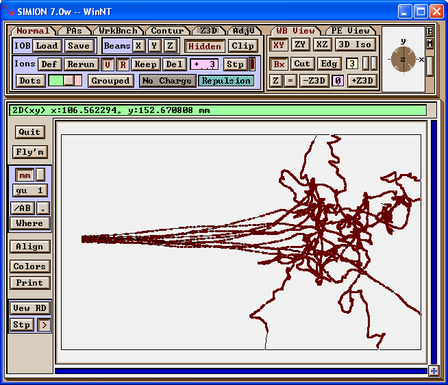
The figure below shows ion trajectories in the HS1 collision model (dots mark collision events). Conditions: ions of mass 200 amu, 15 angstrom collision diameter, and initial velocity to the right at 24 eV colliding against a He background gas with 2 angstrom collision diameter, 4 mTorr pressure, and 275 K temperature. Collisions tend to kinetically cool ions initially. As ions slow down, mean-free-path decreases and the scattering effect increases.
The below figures area plots of ion speed per collision number using the HS1
collision model as well as the earlier dahl_drag.prg and _Trap/INJECT.PRG in
SIMION 7.0 models for comparison. The Ling1997 paper (Figure 4) provides a
similar graph for its collision model under the same conditions. The HS1 and
dahl_drag.prg models are in fairly good agreement in this aspect. However,
these differ from the Ling1997 and _Trap/INJECT.PRG graphs, which are
similar to each other and show almost twice as rapid dampening. (Note: full
details of Ling1997 are not available.) The reduced dampening in the former
models seems partly due to the inclusion of heating collisions from behind the
ions.
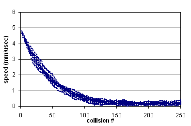
Fig. 63 Figure: Dampening using Collision Model HS1
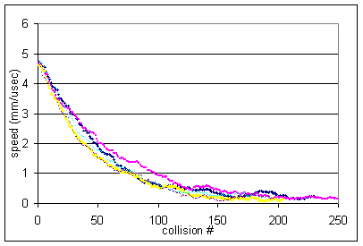
Fig. 64 Figure: Dampening using Collision Model dahl_drag.prg
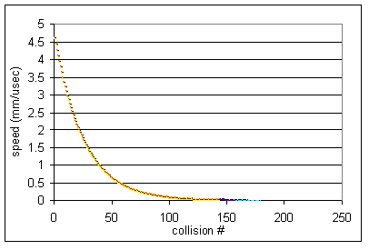
Fig. 65 Figure: Dampening using Collision Model _Trap/INJECT.PRG in SIMION 7.0 (also resembles Ling1997)
Despite these similarities in the above regard, the models can
still be quite different. For example, HS1 model supports a
variable mean-free-path (unlike dahl_drag.prg), and this affects
the frequency of collisions, especially as speeds change. Models
can also handle angular scattering differently (e.g.
_Trap/INJECT.PRG does not provide any angular scattering).
Appendix: Derivation of Mean Relative Speed
This program calculates mean relative speed between the ion and background gas in order to calculate mean-free-path. The following is a derivation of the equation for mean relative velocity.
Compute average relative speed c of a single particle (ion) against a background gas (gas). The background gas is assumed to be Maxwell distributed in velocity.
We start with

where f is the three-dimensional Maxwell distribution given by

such that  .
.
Substituting,

Let  .
.

Convert to spherical coordinates and let  .
.

Let  .
.

To solve this integral, we use

Substituting,
![\begin{align*}
c = & A^{1/2} \pi^{-1/2} a^{-1} \exp(-Aa^2) \\
& (\frac{2Aa^2 + 1}{2A^2}\pi^{1/2}
\exp(Aa^2)A^{1/2}\operatorname{erf}(A^{1/2}a) + (a/A)) \\
& (2A^{-1/2} \pi^{-1/2}) \cdot
\left[ \frac{\pi^{1/2}}{2} (A^{1/2}a + \frac{1}{2} A^{-1/2}a^{-1})
\operatorname{erf}(A^{1/2}a) +
\frac{1}{2}\exp(-Aa^2)
\right]
\end{align*}](_images/math/5040c3f3c93047bd362380f29b8692bf23c2c22b.png)
Let


Substituting gives the result:

This result is in agreement with Ding2002.
Note the following resuts:
As  .
.
Also, as
 .
.
Further, if  , then
 , which is approximately the
average relative speed between the gas particles themselves
(
, which is approximately the
average relative speed between the gas particles themselves
( ).
).
The above results provide a rough justification for the
approximation
 .
.