Potential Array File Types (Comparison)
Potential array files come in a number of different types (.PA, .PA#, .PA0, .PA1, etc. files). How do they differ?
Summary
The simplest of these is the basic potential array (.PA file). It represents the potential at every point on a rectangular grid, stored in a multidimensional array.
A fast adjust array (.PA0 file) is like a basic PA but its electrode voltages can be quickly adjusted (i.e. fast adjusted) without needing to Refine again. It does this by consulting additional electrode solution arrays (.PA1, .PA2, etc.), typically one per electrode, and having the same format as a basic PA, taking an appropriate linear combination weighted by the desired electrode voltages. These arrays are created automatically when the user refines a fast adjust definition array (.PA#), which again is the same as a basic PA except electrode index numbers (1, 2, etc.) not voltages are assigned to electrode points.
Fast adjust arrays do require more memory and refine time, but there are compromises between the two types, using fewer solution arrays if not all electrode voltages need be independent (defined with .PA+ files).
Basic Potential Arrays
A basic potential array, which has the file extension .PA, is the simplest type of potential array. For simpler applications it may be the only type you need. A .PA file is a 2D or 3D rectangular grid–sometimes called a “mesh”–of points in space. Each point in the array defines
a potential – either an electrostatic potential in Volts or scalar magnetic potential in Mags
a flag marking the point as an electrode or non-electrode point.
Typically, when you first create a .PA file, you mark some points as electrodes and specify the potentials on those electrode points. The potentials on the non-electrodes points are initially unknown and are assumed unspecified by the user. In this condition, we say that the state of the array is unrefined, meaning that although the boundary conditions for the Laplace equation have been defined, but the potentials in the array at the non-electrode points do not yet satisfy the Laplace equation under those boundary conditions. However, by running the Refine function, SIMION computes and sets the potentials of the non-electrode points, and we then say that the state of the array is refined.
Once a .PA file is refined, any subsequent edit to it would normally put it in an unrefined state. The nonelectrode points will no longer have the potentials required by the Laplace equation for the new electrode definitions until refined again. There are a few exceptions. We can proportionately scale the potentials of all points in the array by some constant. The linearity of the Laplace equation ensures that the Laplace equation is still satisfied (the array remains refined) after making this transformation.
Fast-Adjust Potential Arrays
A fast-adjust array (or fast adjust base solution array) (.PA0 file) is like a .PA file but more flexible. A .PA0 has the same format as a .PA but except that it has some additional data (specifics are in File Format). The main advantage of .PA0 files is that you can quickly adjust (i.e. “fast adjust”) the electrode potentials without refining again. You can independently change all electrode potentials (not just proportionately scale by the same constant like a .PA file).
When you “fast adjust” a .PA0 file, the potentials inside it are recalculated from a specific linear combination of the potentials in the electrode solution arrays (.PA_, .PA1, .PA2, .PA3, etc. files). There is one electrode solution array per independently adjustable electrode. The .PA1 file corresponds to electrode #1, the .PA2 file corresponds to electrode #2, etc. Finally, the .PA_ file, corresponds to electrodes that are not independently fast adjustable, like a .PA file, and it doesn’t exist if there are no such electrodes. Electrode solution arrays have the same format as .PA files. Each of the electrode solution arrays has its represented electrode set to 10000V and the other electrodes set to 0V, and the potentials of the non-electrode points satisfy the Laplace equation (i.e. they are in a refined state). The linearity of the Laplace equation allows us to quickly determine solutions from linear combinations of individual electrode solution.
You normally don’t need to look at the “electrode solution” arrays, but it can be instructive to do so. Here is what they look like in View for a simple three-element lens:
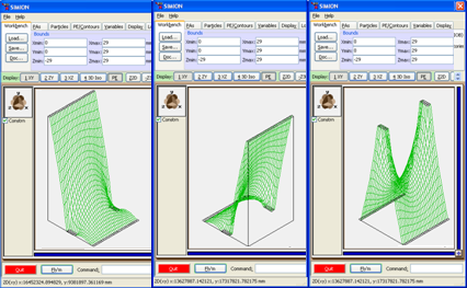
Fig. 22 Figure: Potential energy surface views of (left) .PA1 file, (middle) .PA2 file, (right) .PA3 file.
The .PA0 file and the corresponding electrode solution arrays are not created by you but by SIMION when you refine a fast adjust definition potential array (.PA# file). A .PA# has the same format a a .PA file exception that instead of storing potentials on electrode points, you normally instead store electrode index numbers (positive integers) at those points. The actual potentials that those index numbers correspond to are defined later, after refining. Here’s what the .PA# file used to generate previous three-element lens looks like in Modify:
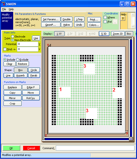
Figure: .PA# file viewed in Modify screen.
Note that the values in the .PA# file are not actual potentials but rather indices (1, 2, 3) to potentials to be defined later during the fast adjust. The .PA0 file contains real potentials.
Unlike a .PA file that may be in an unrefined or refined state, a .PA# (which you edit) is always considered unrefined, and .PA0 file (which you never edit apart from fast adjusting) is always considered refined.
Once a .PA0 file is generated, the .PA# file is no longer used except if you want to edit the geometry in the .PA# file and re-refine again.
The typical process of using .PA0 files in SIMION is:
Create the .PA# file in Modify or by another means (e.g. GEM/STL).
Refine the .PA# file (generates .PA0, .PA_, .PA1, .PA2, .PA3, etc. files).
Fast Adjust the .PA0 file.
Add the .PA0 file to your workbench and fly particles through it.
When you use a .PA0 file, SIMION automatically takes care of superimposing the fields. You don’t ever need to touch the electrode solution arrays.
Which to use?
The main reasons use to a .PA0 file rather than a .PA file are when
electrode voltages need to be changed during a Fly’m (e.g. time dependent voltages like pulses or RF waveforms) or controlled by a user program.
electrode voltages need to be quickly changed (e.g. tuning voltages).
In simpler cases of time-dependent fields (SIMION Example: rfdemo),
proportionally scaling a field with a basic .PA can still be used
(e.g. efield_adjust segment), but this is a special case.
Some examples of fast adjust arrays:
RF fields (SIMION Example: quad, SIMION Example: octupole, and SIMION Example: trap)
time dependent voltages (SIMION Example: buncher),
static field examples where voltages need tuned (SIMION Example: einzel).
SIMION Example: misc (test3d.pa) is an example of a basic PA.
Reasons for still using a basic PA:
It’s simpler.
It’s only one array in RAM (less RAM use).
It’s only one array on disk (less disk use).
It’s only one array to Refine (less time to Refine).
Marginally may be more accurate fields in some scenarios (less “fast adjust” numerical math).
Fast-Adjust Potential Arrays with Multiple Proportional Scalable Electrodes
For a system containing many electrodes with different voltages, we could choose to represent it with either a .PA or .PA# file. If we use a .PA file, the electrode voltages can only be proportionately scaled but on the up-side it only requires a single array and therefore is very efficient. If we use a .PA# file, we have the added flexibility of independently adjusting all electrode voltages at the expense of generating many electrode solution arrays that potentially take a lot of time to refine and consume a lot of memory. A compromise between these two options is to augment the .PA# file with a .PA+ file. A .PA+ file, which is a regular text file not an array, causes the electrode indices in the corresponding .PA# file to be reinterpreted such that sets of electrodes are grouped (where groups might overlap) and each group is independently proportionately scalable. Each group generates only one electrode solution array. .PA+ files were added in SIMION 8.0.3. A .PA+ file is not needed if you have only one of these groups: .PA# file electrode points that are not low positive integers are automatically interpreted as belonging one such group and are written to a .PA_ electrode solution array file.
For further details, see Additional Fast Proportional Scaling Solutions.
Other Uses of Potential Arrays (besides Storing Potential)
Generally, a potential array (.PA) represents a scalar field. That is, it represents some number that varies over a 2D or 3D space. Normally, this number is understood by SIMION to be a potential. However, as we saw with .PA# files, which are really just .PA files with a different name and interpretation, there is no hard requirement that this be the case. You could store any other scalar variable in the array (e.g. index numbers, temperature, pressure, the X component of a velocity vector, charge density, etc.) There are libraries in SIMION 8.0 SL Libraries and SIMION 8.1 Lua PA API (simion.pas) for reading and writing potential arrays, so you can use potential arrays for your own purposes. The Poisson Equation solver, for example, uses arrays to represent a charge density distribution in space. The HS1 (SIMION Example: collision_hs1) and SDS (SIMION Example: collision_sds) collisions models allow pressure, temperature, and components of the gas velocity vector to be represented as arrays–either as real SIMION potential arrays or as arrays represented as Lua tables (see also SIMION Example: cfd). The field_array (SIMION Example: field_array) example represents x, y, and z components of a field vector in space.