Lambert Cosine Emission
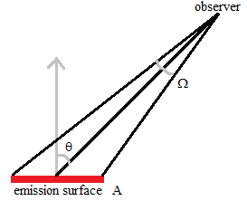
Fig. 27 Emission surface observed from angle  relative to surface normal, and solid angle
  .
.
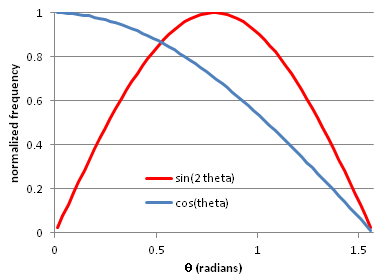
Fig. 28 Normalized observed current per solid angle (blue)
and emitted current per  (red) v.s. .
A Lambertian emitter has the same brightness (i.e. current per area per
solid angle) when observed from all angles.
A Lambertian emitter therefore follows Lambert’s cosine law,
which is to say that the angular current density
(i.e. current per solid angle) observed from
an angle (relative to the surface normal) is
proportional to  .
That is because the emission surface appears to have a size proportional
to
.
That is because the emission surface appears to have a size proportional
to  from a vantage point of that angle.
The angular current density is independent of the angle
from a vantage point of that angle.
The angular current density is independent of the angle  of rotation around the surface normal.
FLY2: See SIMION Example: particles (lambert_cosine.fly2) (added in 2015-07-15) for an example of generating a Lambert Cosine distribution of emission in a Monte Carlo Method fashion in a FLY2 file.
Sampling:
If all rays traced in a beam represent the same current, we can sample a
random ray from a Lambert cosine distribution in Monte Carlo fashion as follows.
The probability of a ray with angle is  for
for
 .
This gives a random variable
.
This gives a random variable
 , where
  is a uniformly
distributed random variable between 0 and 1.
The probability of a sampling a ray with angle is
proportional not to but to
is a uniformly
distributed random variable between 0 and 1.
The probability of a sampling a ray with angle is
proportional not to but to
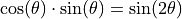 since
the solid angle covered by all observers (at any ) with
angle is proportional to
since
the solid angle covered by all observers (at any ) with
angle is proportional to  .
Inverting this distribution,
.
Inverting this distribution,
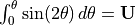 , implies
 .
So, we have the random variable
.
So, we have the random variable  .
.