Particle Initial Conditions¶

Lambert Cosine Emission

Overview¶

Before doing Particle Trajectory Calculations, the initial conditions of the particles must be defined, such at position, velocity, mass, and charge at time t=0. Initial conditions on particles can be defined in various ways in SIMION. You can use an ION File, a FLY File, a FLY2 File, or a user program.

The ION File provides a very general method and just consists of a list of particle parameters in a straightforward “comma-separated-value” (CSV) text format as described in Section F.6 “Ion Definition File” (SIMION 8.0 manual), p. 8-6 (SIMION 7.0 manual), or ION File. There are a number of ways to create this file from external programs or from SIMION itself.

The FLY File allows a linear sequence of particles to be defined rather easily via the SIMION GUI, but it can only be used if your particles can be defined as a linear sequence, and it is not easy created from an external program. Therefore, FLY files are only useful in limited circumstances. FLY files are built using “Define Ions by Groups” in the SIMION ion definition screen.

The FLY2 File (new in SIMION 8.0) allows particles to be defined in a very flexible but simple way. FLY2 is a replacement for the FLY format. A FLY2 file can also be converted into an ION file.

The old .fly format is a subset of the capabilities in the .fly2 format. Any .fly file can be automatically converted (reversibly) into a .fly2 file (but not vice-versa), and any .fly2 file can be automatically converted (irreversibly) into an .ion file. This conversion is done just by switching “How are particles defined?” on the Particles Define screen.

A workbench user program (initialize segment) can define particle parameters at the start of ion flight. User programs are just as flexible as ION files (e.g. it is even possible for a user program to essentially load and use an ION file), but they are even more flexible since ion parameters can be calculated in the middle of the simulation or parameterized by adjustable variables. They can require a bit more experience to create though and are not always needed.

An ION itself can be generated in many ways:

Create with the SIMION GUI (“Define Ions Individually”)
Create from a FLY/FLY2 file
Create from SIMION Data Recording output (click “Ion” button for .ION file format)
Create from Excel or any other external program (e.g. C, Perl, TRIM, etc.)
Virtual Device includes some routines for generating .ION files for common beam types.

Creating the ION file from the SIMION GUI is done with “How are particles defined? Individually (.ION)” (or “Define Ions Individually” in version 7) on the partial definition screen. It would b e tedious to use if you have many particles. Still you can use any other tool. You might be more familiar with Excel or you might generate the initial ion parameters from another simulation program (e.g. TRIM).

User Programming Examples¶

Uniformly randomized cone angle¶

The follow PRG program uniformly randomizes the directions of ions within a certain cone angle. A cone vertex angle of 180 degrees achieves a completely random direction. This code is actually an improvement on SIMION’s random.prg/random.sl examples, which generate random direction that are not entirely uniform. A uniformly random direction is achieved by applying transformation derived from the fundamental transformation law of probabilities.

; PRG program to randomize ion direction within a cone.

; angle in degrees of cone vertex (use 180 for all directions)
DEFA vertex_angle 180

SEG initialize
   ; get ion's specified velocity components in polar form
   RCL ion_vz_mm
   RCL ion_vy_mm
   RCL ion_vx_mm
   >P3D
   STO speed RLUP
   STO az RLUP
   STO el RLUP

   ; compute uniformly randomized direction from +Y axis.
   ; c = 1 - cos(vertex_angle * PI / 180)
   1 RCL vertex_angle 3.141592 * 180 / COS - STO c
   ; el2 = arccos(1 - rand() * c) * 180 / PI + 90
   1 RAND RCL c * - ACOS 180 * 3.141592 / 90 + STO el2
   ; az2 = rand() * 360
   RAND 360 * STO az2

   ; convert to rectangular coordinates
   RCL el2
   RCL az2
   RCL speed
   >R3D

   ; rotate center back to +X axis.
   ; then rotate center back to original direction
   -90 RCL el + >ELR
   RCL az >AZR

   ; save new velocity vector
   STO ion_vx_mm RLUP
   STO ion_vy_mm RLUP
   STO ion_vz_mm RLUP

Here is an equivalent FLY2 file (which avoids user programming):

standard_beam_define {
   n = 100,
   x = 0, y = 0, z = 0,
   direction = cone_distribution {
     axis_direction = {1, 0, 0},
     vertex_angle = 180
   }
}

Here is an equivalent way to do that in Excel: simion_cone.xls.

Lambert Cosine¶

See Lambert Cosine Emission.

Procedure for creating a .ION file in Excel¶

The follow procedure is recommended for building an ION file in Excel:

Create and save a simple .ION file using SIMION (View | Def | Define Ions Individually | Save). This will be used as a template so that you don’t have to create the file entirely from scratch.
Load the .ION file into Excel. When prompted during import, choose “delimited” format and “comma” delimiters (i.e. comma-delimited).
Edit the data in Excel. You can even define ions using formulas.
Save the file in Excel. Do this with “Save As” and choose “CSV (comma delimited) (*.csv)”. Name it with a .ion extension (e.g. “hello.ion”), adding double quotes around the filename so that Excel doesn’t try to add a .csv extension to the file name.

Note that a little care is required since Excel otherwise expects CSV file names to have a “.csv” extension rather than a SIMION “.ion” extension. If you are not careful, Excel will save/read your file in ‘’‘tab-delimited’‘’ rather than comma-delimited format. Also, if you need to save any formulas, you must save a copy of your spreadsheet in a more intelligent format (e.g. native Excel .xls format).

For an example, see simion_cone.xls (updated on 2006-01-30 so that the angle is uniformly random).

If you wish to express velocity directions as vectors (vx,vy,vz) rather than angles, the conversion formulas in Excel are

"Azimuth angle (az)"
=DEGREES(ATAN2(X, -Z))

"Elevation angle (el)"
=DEGREES(ATAN2(SQRT(X^2 + Z^2), Y))

Note the the order of operands of the ATAN2(x,y) function in Excel are reverse that in the math.atan2(y,x) function in Lua.

Flying ions in the reverse direction or other ion transformations¶

The following procedure can be used to fly ions in the reverse direction of a previous simulation. It can be a useful check of accuracy. Similar methods can be used for other situations as well, such as secondary emissions.

For example, consider SIMION’s TOF example (SIMION Example: tof). The ions start at the source at and hit the detector. Given ion conditions at the source, SIMION calculates the ion conditions at the detector. But, what if we already have the conditions at the detector (e.g. from SIMION’s data recording) and want SIMION to instead calculate the conditions at the source, or something similar?

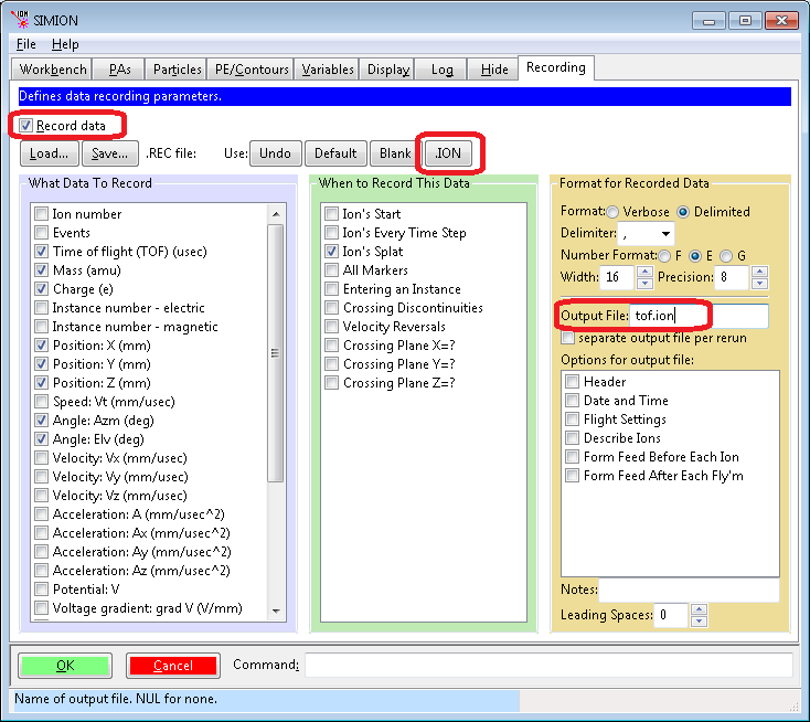
We start as usual by calculating ion conditions at the detector with SIMION’s Data Recording feature. In the Data Recording screen, enable Record data, click the .ION button so that SIMION records data in the same format as the (.ion file), and specify an Output File (or to dev/file in SIMION 7.0) named tof.ion. Note that data is recorded When Ion's Splat (against the detector).

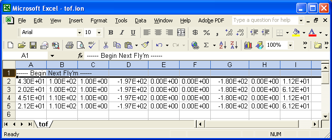
Fly the ions. SIMION writes the file tof.ion containing the ion conditions at the detector. This information is also displayed in the Log window tab.

Now, we want to reverse this process. We first need to reverse the ion conditions (e.g. their velocity direction) just obtained. We can do this by editing the .ION file in Excel. When loading in Excel, be sure to specify “delimited” format and the “comma” delimiter.

Delete the first comment row (since SIMION will trip on it). Columns G and H are the azimuth and elevation angles (in degrees) respectively. To reverse the direction add (or, equivalently, subtract) 180 degrees to the azimuth angles and multiply the elevation angles by -1 (see figure of coordinate system in the SIMION User Manual– page L-10 in SIMION 8.0/8.1, I-6 in SIMION 7.0).

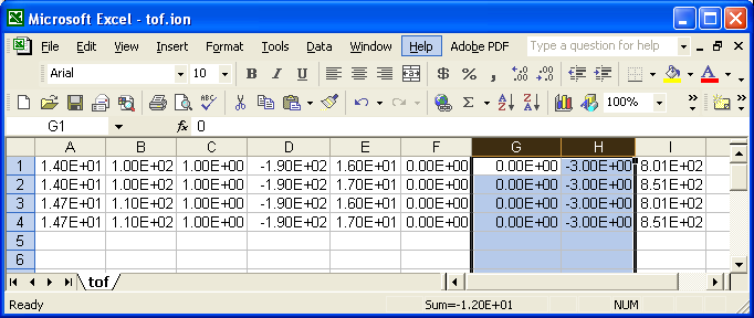
Now save. Be sure to save it in the “CSV” (comma-separated-value) format. Include double quotes around the filename so that Excel uses the filename exactly as specified (not try to append a “.csv” to it).

Now, in the SIMION Particles Define screen, load the ION file. Ensure that the coordinates are defined relative to the workbench (in mm), as these are the coordinates that SIMION Data Recording uses. You should also clear the Output File box on the Data Recording screen so as not to overwrite your newly modified ION file.

Refly.

Note the similarity in trajectory shape compared to before. One property of electrostatic fields is that they are reversible in this way–a property that we make use of here. How well this property holds provides measure some of simulation accuracy.

You might use similar methods to acquire data recording data on some plane and then restart the ions at the same position (maybe reversing, randomizing, or changing the ions in a sort-of like a secondary emissions effect–SIMION Example: secondary). You might also use this type of method to transform ion data to and from another simulation program. One might alternatively use user programs to do the ion transformations.

Virtual Device also has some functions for transforming SIMION .ION and Data Recording files.

A simpler way to do all the above is to just attach a workbench user program such as this (via the “User Program” button on the SIMION 8.0/8.1 Particles tab):

simion.workbench_program()
local nsplats = {}
function segment.other_actions()
  -- If particle splatting for the first time, reverse velocity
  -- and disable splat.
  if ion_splat == -1 and not nsplats[ion_number] then
    ion_vx_mm = -ion_vx_mm
    ion_vy_mm = -ion_vy_mm
    ion_vz_mm = -ion_vz_mm
    ion_splat = 0
    nsplats[ion_number] = (nsplats[ion_number] or 0) + 1
  end
end

Here is another version:

-- reverse particles when they hit a test plane
simion.workbench_program()
local TP = simion.import 'c:/Program Files/SIMION-8.1/examples/test_plane/testplanelib.lua'
local test1 = TP(80,0,0, 1,0,0, function()  -- test plane at x=80mm
  -- reverse particle velocity when it hits a test plane.
  ion_vx_mm,ion_vy_mm,ion_vz_mm = -ion_vx_mm,-ion_vy_mm,-ion_vz_mm
end)
function segment.tstep_adjust()  test1.tstep_adjust() end
function segment.other_actions() test1.other_actions() end
-- see also "examples\test_plane"

The relationship between 3D rectangular and polar coordinates is as follows:

r3 = sqrt(x*x + y*y + z*z)
r2 = sqrt(x*x + z*z)
azimuth   = atan2(-z, x) * (180 / math.pi)
elevation = atan2( y,r2) * (180 / math.pi)

(Note: atan2(a, b) is similar to atan(a/b)–see math.atan2().)

Mass and Charge Limits¶

SIMION 8.1.1.13 made these expansions to particle definition limits:

Maximum mass changed from 1E+9 u to 1E+100 u.
Maximum charge changed from 9E+3 e to 1E+100 e.
Maximum KE changed from 9E+9 eV to 1E+100 eV.

In earlier version of SIMION (8.0), one workaround is to fly particles with lower mass, charge, and KE that give an equivalent trajectory (though a time-of-time differing my some factor). Note that multiplying the mass, charge, and KE by some factor gives the same trajectories but different TOF in an electric field.


[Optional] Your name:	email:	phone: