First Uniqueness Theorem
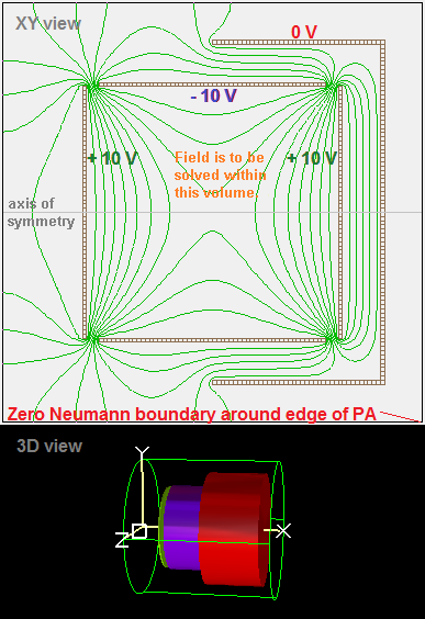
Fig. 74 Figure 1a: 2D cylindrical PA containing some electrodes of various voltages. Potential contour lines (green) are also shown. (This is “first_uniqueness.gem” in SIMION Example: misc in SIMION >= 8.1.1.30.)
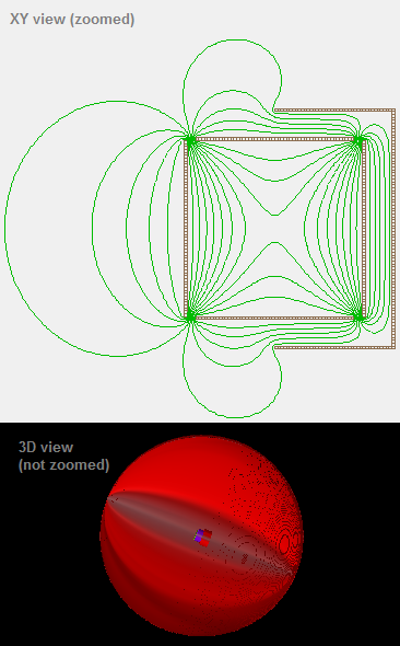
Fig. 75 Figure 1b: Same as Figure 1a but with huge grounded sphere surrounding electrodes. (This is “first_uniqueness_cage.gem” in SIMION Example: misc in SIMION >= 8.1.1.30.)
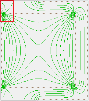
Fig. 76 Figure 1c: Same as Figure 1a but the PA has been cropped (Modify “Crop” function) to remove all PA empty space surrounding the cylinder. Observe field distortions on upper-left corner (highlighted in red box).
Motivation: To obtain accurate electric field calculations, proper attention must be paid to boundary conditions. Boundary conditions are what constrain the solution to partial differential equations like the Laplace Equation, which otherwise have an infinite number of solutions. In SIMION, the electric field is determined from the electric potential throughout some volume of space, which it in turn finds by solving the Laplace Equation. The boundary conditions on the Laplace equation typically take the form of specifying the values of potential (or some other constraint such as the values of the derivatives of potential) that are known over the surface enclosing that volume (the boundary surface). If there is exactly one solution to the field, we say that this solution is unique. Theorems that tell us what types of boundary conditions give unique solutions to such equations are called uniqueness theorems. This is important because it tells us what is sufficient for inputting into SIMION in order for it to even be able to solve an electric field.
The first uniqueness theorem: The first uniqueness theorem is the most typical uniqueness theorem for the Laplace equation:
First Uniqueness Theorem: “The solution to the Laplace Equation in some volume is uniquely determined if [the potential voltage] is specified on the boundary surface.” [so-called Dirichlet Boundary Conditions] (Griffiths, 1999)
Sections of the boundary surface that have known potential are called Dirichlet Boundary Conditions. Often these boundary conditions consist of the shapes and potentials of the surfaces of metal conductive electrodes that bound the volume. These things can often be well controlled experimentally by machining the electrodes to the proper shape and holding them to a desired electric potentials via power supplies. We typically use conductive, rather than insulative or semiconductive, material here because conductors maintain a uniform potential over their entire surfaces (there’s another theorem that says this).
Implications on SIMION: The first uniqueness theorem implies that SIMION can calculate unique values of non-electrode point potentials within any volume that is surrounded entirely by a “closed” surface of electrode points. By “closed” we mean that if you fill the system with water, it won’t leak. In Figure 1a, the center cylindrical region surrounded by +-10 V electrodes is not, strictly speaking, closed because there are gaps between the electrodes, but it would be closed if these gaps were filled with electrode points representing Dirichlet conditions. Now, we cannot physically fill these gaps with conductive material because electrodes with dissimilar potential will arc and thereby eliminate the potential difference between them if they touch (or even get very close). To say that we fill these gaps with electrode points rather would mean that there is insulative or semiconductive material, or vacuum, in the gaps physically and we just happen to know exactly what the potentials at those points in the gap are, so we define them with Dirichlet conditions, which are represented in the SIMION simulation as electrode points, even though they aren’t really conductive electrodes. We will see later that in practice we don’t need to do this, but it’s an instructive thought exercise.
Other guarantees of uniqueness (Neumann boundaries): The first uniqueness theorem does not describe the only conditions that can ensure a unique solution to the Laplace equation (it is not the only uniqueness theorem). The Laplace equation still has a unique solution if part of this boundary is instead defined by a Neumann Boundary Condition, in which the normal derivative of potential (not the potential itself) on the boundary is specified. Neumann boundary conditions occur, for example, on mirror planes, such as SIMION X/Y/Z mirror planes as well as any axis of symmetry (like in Figure 1a), in which case this derivative is zero. PA edges of non-electrode points (also seen in Figure 1a), even if non-mirrored, are treated as a Neumann boundary condition of zero (this is true in SIMION 8.1 and is nearly the case in previous versions too–see Neumann Boundary Condition). Therefore, every SIMION PA has a closed boundary (the edge of the array) consisting of some combination of Dirichlet and Neumann boundary conditions, and SIMION will go on to calculate it, but whether these Neumann boundary conditions assumed here are valid approximations of your system is something you’ll need to determine (see p. 6-3/6-4 of the 7.0/8.0/8.1 SIMION User Manual).
The astute reader may notice that if the entire PA edge is Neumann
and there are no electrodes inside to constrain the volume to
particular voltage (i.e. the entire PA is empty), then the potential inside
the entire PA will be some unknown constant  ,
but the field will be zero everywhere (since
,
but the field will be zero everywhere (since  = 0).
If all points in the array are non-electrode points of a certain voltage,
they will remain unchanged upon Refine.
Yes, occasionally empty PA’s are in fact useful.
= 0).
If all points in the array are non-electrode points of a certain voltage,
they will remain unchanged upon Refine.
Yes, occasionally empty PA’s are in fact useful.
Why a boundary with holes might still be considered closed: Technically, we can’t ignore the treatment of the boundary conditions outside the cylinder (Figure 1a) when solving the potentials within the cylinder because of the small holes in the boundary that allow fields outside the cylinder to leak inside. However, it happens to be the case that the potentials along these gaps are fairly well defined regardless what the fields may be outside. So, to some extent the outside doesn’t matter. The potentials within the gaps must vary continuously from +10 V to -10 V along a small distance, so this fairly well constrains what the potentials are in this region regardless of what is outside. In fact, we observe in Figure 1a that the potentials within the cylinder are nearly symmetric between left and right sides despite the fact that the fields are not symmetric outside due to the additional electrode on the right. The gaps between the +-10V electrodes could even be filled with electrode points (Dirichlet conditions) that vary linearly (which is only an approximation) from +10 V to -10 V, and this will barely distort the field inside. In this case, we see that a nearly equivalent system is closed, so the first uniqueness theorem will largely still apply to the inside of the cylinder despite the gaps.
Treatment of boundaries on PA edges: In Figure 1a, the validity of the Neumann condition near the PA edge is questionable and generally wrong. You see the potential contours touch the boundary at 90 degree angles (as required by the Neumann boundary condition), and their exact shape will depend on the position of the PA boundary. Fortunately this might be a region we don’t care much about, but it still might leak through the gaps to some degree. It may be more realistic to enclose the cylinder with a large (nearly infinite size) sphere of 0 V, as shown in Figure 1b. This certainly does alter the potentials outside of the cylinder, but the potentials inside the cylindrical are largely unaffected except to a small extent near the gaps. Even the potentials between the cylinder and surrounding electrode on the right are largely unaffected except to a small extent on the open end. This gives us greater confidence that the uncertainty about the boundary may not be that important.
The ground chamber: Note further that an infinite grounded sphere is itself only an approximation of the reality of the electrostatic environment around your system, and this environment might not be known. In order to address this and other issues, most particle optics devices are placed inside a Ground Chamber, which is a closed (or nearly closed) grounded metal surface around your system. For compactness, the ground chamber is typically fairly close to your system (unlike the large infinite sphere) though not so close to significantly distort fields in the inner volume of interest. It may look like the right 0 V electrode in Figure 1a but extended to enclose the left side as well. As we’ve seen above, the exact shape of the ground chamber may or may not be important, but since it is small and potentially affects the fields, it is often easy and desirable to include the ground chamber in your simulation. The ground chamber forms a complete or nearly complete Dirichlet boundary, ensuring the fields within the chamber are uniquely determined by the first uniqueness theorem. The ground chamber (ground can) is also mentioned on p. 6-4/6-3 of the SIMION 7.0-8.0 SIMION User Manual. It’s basically a Faraday cage (Wikipedia: Faraday_cage).
Use of empty space on PA edges: If you have no ground can, it can be recommended to at least include some empty surrounding space in your PA to allow fringe fields to be more realistic. Observe Figure 1c, which is the PA in Figure 1a but has been tightly cropped so that no surrounding space has been included in the array. Observe that fields surrounding the gap are more distorted compared to what is seen in both Figures 1a and 1b because this is artificially imposing an (unrealistic) Neumann condition right at the gap location.
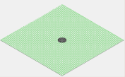
Fig. 77 Figure 2a: 2V circular electrode enclosed entirely with Neumann boundaries on the PA edges. All potentials are calculated as 2V, which is probably not desired.
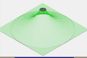
Fig. 78 Figure 2b: 2V circular electrode enclosed with 1V circular Dirichlet boundary. All potentials are calculate between 1-2V as expected. Potentials in the ignored outside area are 1V due to Neumann boundaries on the PA edges.
Why a PA with a single electrode has no field: Users starting out with SIMION sometimes put a single electrode with non-zero potential in a PA and wonder why it has no electric field. Figure 2a on the right is a simple such example involving a centered 2V electrode with no other electrode points. SIMION treats the external boundary on the PA edges as Neumann conditions. The Laplace Equation (and SIMION) calculates a unique solution to this problem, which is 2V on all non-electrode points. This might not be what you intended. You probably expected potentials to decrease to zero by the 1/r relationship of Coulomb’s Law. But that is not the boundary condition you entered. If you instead add a huge ground sphere (Figure 2b, as was also done in Figure 1b), you would see that effect. The calculation of 2V is not entirely unrealistic though if you consider that the definition of “ground” potential is relative. If you likewise apply 2V to the huge sphere and rename that “ground”, you will observe no fields throughout the entire volume. Observe also that the Laplace equation can be thought of as an averaging process, and the potentials calculated on the non-electrode points will always be somewhere inside the interval defined by the minimum and maximum potentials on the boundary points (which here is [2V,2V]).
Further look on the affect of empty space in a PA: Figure 3 shows a milder but still potentially problematic scenario. This is of two parallel plates offset to one corner inside a PA whose edges are entirely non-electrode points. Here, the parallel plates are Dirichlet boundaries and the PA edges are Neumann boundaries. This has a unique solution and SIMION does calculate it. However, do the Neumann boundary conditions represent physical reality? Probably they don’t except to the extent that as you approach infinite distance, not only might potential approach zero, but the normal derivative of potential would approach zero too, so the Neumann boundaries on the PA edges approximate the slope of potential at infinite distance except that this constraint has just been moved closer, to the PA edges, which is an approximation. The approximation might be good enough. Observe that the calculated potentials in the region between the plates are no different than you would expect, and even the fringe regions immediately near the plate openings bear resemblance to that of an infinite ground sphere surrounding the system. However, at the PA edges, the potential contours lines are obviously unrealistic: the contour lines tend to be more perpendicular to the PA edges (a Neumann condition constraint) than exist theoretically if a infinite ground sphere were assumed. Since the plates are offset with respect to the PA edges, one sees a clear asymmetry in the equipotential contour lines, which also is not expected if the system really did have symmetry. This shows that the amount of empty space around your system can affect the contours. It also shows the uncertainties that a ground chamber can avoid.
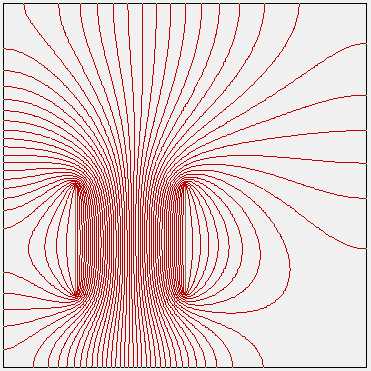
Fig. 79 Figure 3: Parallel plates offset to one corner in a PA enclosed entirely with Neumann boundaries on the PA edges. Equipotential contour lines are shown.
More examples:
SIMION’s einzel\einzel.pa# and magnet\mag90.pa# examples
demonstrate partly open systems (Neumann boundaries).
These are examples where things like Figure 3 can be ok.
Memory limits of an infinite sphere: If you do happen to need a large infinite ground sphere (or anything like that) but are running into memory limitations (e.g. 3D simulation), you might consider using an approach with nested arrays like that seen in Field Emission.
Other Uniqueness Theorems
There is a “second uniqueness theorem” that says that the solution to the Laplace equation is uniquely determined in the volume if the boundary surface consists of conductors each with a known total charge. This is not typically utilized directly in SIMION since more often you know the conductive electrodes’ voltages (controlled by power supplies) rather than the charges, but one may sometimes have a Floating Conductor. One can also utilize the field information surrounding some region to derive the total charge in that region (see Gauss’s Law and Charge-Capacitance Calculation), which, if assuming negligible space charge, can be ascribed to the electrodes in that region.
Poisson Equation
The uniqueness theorems for the Poisson Equation is similar
to that of the Laplace Equation except that in addition
the distribution of space-charge density
throughout the volume ( ) is also required to constrain
the solution.
If the volume contains linear dielectric material,
then the shapes and dielectric constants of that material are also required
(Griffiths Problem 4.35).
) is also required to constrain
the solution.
If the volume contains linear dielectric material,
then the shapes and dielectric constants of that material are also required
(Griffiths Problem 4.35).
Terminology
The term “uniqueness theorem” is also seen elsewhere more generally where some theorem proves that some object is uniquely determined by a constraint. See Mathworld: Uniqueness Theorem and Wikipedia: Uniqueness_theorem.
See also
SIMION User Group discussion 346 comments by Bud and others.
Griffiths Problem 5.54 seeks to prove the uniqueness theorem “If the current density
 is specified throughout a volume V,
and either the potential
is specified throughout a volume V,
and either the potential  or the magnetic field
  is specified on the surface S of V, then the magnetic field is uniquely
determined throughout V.”
is specified on the surface S of V, then the magnetic field is uniquely
determined throughout V.”