Multiple PAs¶

It is simplest and least error-prone to model your entire system as a single PA in SIMION. Refining a PA solves the Laplace Equation within it, so if your entire system is within a PA, the Laplace equation will be solved globally throughout your entire system. However, in some cases a single PA is not ideal. It may require too many grid points (too much memory) to achieve the required accuracy. For example, there may be a region in your system with important tiny details requiring a high density of grid points, and PA’s have a uniform density of grid points throughout.

One way to greatly reduce the number of grid points is to use a PA with a certain symmetry (e.g. 2D cylindrical or 2D planar, possibly with mirror planes). However, often a system lacks such symmetry. Sometimes a system nearly has such symmetry except for a small feature, in which case such symmetry cannot be used except maybe as an approximation.

As an optimization, SIMION allows you to place multiple PAs into a workbench. Each PA is Refined independently, which means that SIMION treats each PA as a completely independent system. The Laplace equation is solved independently on each PA rather than once globally over the entire system. When an particle flies through the workbench, at most one electrostatic PA instance (the highest priority one) containing the particle is seen by the particle (described in Overlapping PA instances).

Obviously, there are caveats to breaking a system into multiple PAs. You need to ensure that the individual field calculations are identical to the single field calculation. Mainly, you need to ensure that the Laplace equation remains satisfied on and between the boundaries of the smaller potential arrays by appropriate boundary conditions on the edges of the PAs. It helps to be familar with the properties of the Laplace Equation such as the First Uniqueness Theorem. In general terms, the fields must “match up” between PA instances.

The method: If you want to use multiple PAs, it is recommended that you first simulate the system as a single PA as a starting point. Use that to observe the fields and fringing effects to determine where it is appropriate to cut the PA so that the Refine calculation is still valid. There may be Dirichlet Boundary Conditions or Neumann Boundary Condition, such as a field-free region, which can serve as a convenient location in which to place an edge of a PA that also has that same boundary condition. Whatever you do, the fields in the multi-PA system must resemble the fields in the original single-PA system. There is no hard and fast rule of how to do this, as it depends on the type of geometry you have.

SIMION Example: quad in SIMION is a good example of using multiple PAs. This system has almost 2D planar symmetry on the long rods, but the entrance and exit lenses break that symmetry, so a 3D array would typically be needed. It would be desirable, therefore, to cut the system into three potential arrays: a 3D entrance lens, a 3D exit lens, and the rods with 2D planar symmetry (at high resolution). To do this, the system was first modeled as one big (but course) potential array. The result provided an indication of how far the fields penetrate through the entrance and exit. The system was then cut into three potential arrays at locations far enough away from the entrance and exit such that the fields are largely 2D symmetric along the length of the rods.

SIMION Example: bender_cut (added in 8.0.5) is an excellent example of splitting two lenses that join at a 90 degree angle into two arrays that overlap enough such that the calculated fields are valid in the center of the overlap. The fields calculated on the ends of both arrays are invalid, but these regions can be removed with the “Crop” function on refined arrays or (in SIMION 8.1) with a user program like in Overlapping PA instances to ignore fields in these regions.

SIMION Example: field_emission (added in 8.1.1.0) illustrates using nested coarse and fine arrays, while transferring boundary point between them in an automated way. See also the screenshot in Field Emission.

SIMION Example: bradbury_nielsen_grid uses a technique to make fields match up between fine and coarse PA instances, even when RF voltages are being applied in the PA instances. This is done by defining Dirichlet conditions (expressed in SIMION as electrodes) on the edges of both PA instances and using this user program to appropriately set potentials on those boundary conditions so that the fields are the same on both sides of those boundary conditions, over all time.

For details, see the following:

SIMION 8.0 Manual Section 7.2.4 under “Interpolating Electrostatic Fields Between Instances” (~p.7-10) (or p.7.8 of the SIMION 7.0 manual)
SIMION 8.0 Manual Section 9.2 (or SIMION 7.0 Manual, p. 9-2 to 9-4) “Advanced Strategies and Tactics - Doing more with Array Instances”
quad example in SIMION 8.0 or 7.0
SIMION 8.0 Manual Section 7.6.2 “The Copy Button” (or SIMION 7.0 Manual, p. 7-38 to 7-39)

Programmatically Controlling PA Instance Priority¶

The PA instance priority can be effectively controlled from a workbench Lua program. One case where this is especially helpful is if two PAs (e.g. A.pa and B.pa) partly overlap and are refined independently like this:

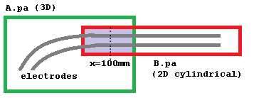
If the boundary conditions on the edges of these two PAs are not accurately defined, the fields near the boundaries will not be accurate either; however, it may be that futher inward from the boundaries the fields are quite good. In such case, we may want to imagine a line through the center of the overlap region and use A.pa for points to the left of that line and B.pa for points to the right of that line. It is not normally possible to achieve this by ordering the PA instance priorities (via the L+/L- buttons on the View screen PAs tab). One solution is to use the Crop function (on Modify screen Issue-I313 or simion.pas pa:crop()) to remove the unwanted overlap region from one or both of the refined PAs (as done in SIMION Example: bender_cut). A quicker and more flexible solution is to use a workbench Lua program to redefine which field (A.pa or B.pa) is seen as a function of position.

The cleanest way to do this is with the new segment.instance_adjust() in SIMION 8.2. This segment effectively allows you to suppress certain regions of any PA instances, causing SIMION to query the next PA instance in the PA instance order. See segment.instance_adjust() for details.

simion.workbench_program()
function segment.instance_adjust()
  if ion_instance == 2 then
    if ion_px_mm > 10 then
      ion_instance == 0  -- suppress
    end
  end
end

Another way to do this, available in SIMION 8.1, is to override the efield_adjust (or mfield_adjust) segment and from there query the PA instance objects.

simion.workbench_program()

local function field_of_instance(instance_number)
  return function(x,y,z)
    local Ex,Ey,Ez = simion.wb.instances[instance_number]:field(x,y,z)
    if not Ex then return 0,0,0  -- outside of array volume
    else return Ex,Ey,Ez end
  end
end
local function efield_adjust_of_instance(instance_number)
  return simion.experimental.make_efield_adjust(field_of_instance(instance_number))
end

local e1 = efield_adjust_of_instance(1)
local e2 = efield_adjust_of_instance(2)
function segment.efield_adjust()
  if ion_px_mm < 100 then
    e1()
  else
    e2()
  end
end

The above uses the simion.experimental.make_efield_adjust() convenience function (8.2EA-20140319(8.1.2.7)) (or simion.experimental.make_mfield_adjust() for magnetic fields). Prior to 8.1.2.30, replace the function field with field_wc (its older name).

Now, the field function normally just reads from the PA instance, without concern for time-dependence such as the effects of segments like fast_adjust. In 8.2EA-20170127, you can pass the current time (ion_time_of_flight) as the fourth parameters to the field function, and that will cause these segments to be invoked for the current particle and given time. That will behave more like the instance_adjust, except here the field is still being calculated and then recalculated, which isn’t as clean or simple to understand.

It is also possible to pass the field function a table of voltages rather than a time, which somewhat recreates the functionality of the fast_adjust segment. There’s probably no longer much need to do this, but here is the code:

simion.workbench_program()

-- Gets field function f for given PA instance number.
-- f(x,y,z) -> Ex,Ey,Ez.  Units in workbench mm and V/mm.
-- An optional function adjust(t, instance_number) acts similar
-- to a fast_adjust segment but updates the table t with electrode
-- voltages and is passed the PA instance number via the argument `instance_number`.
local function field_of_instance(instance_number, adjust)
  local t = adjust and {} or nil
  return function(x,y,z)
    if t then adjust(t, instance_number) end
    local Ex,Ey,Ez = simion.wb.instances[instance_number]:field(x,y,z, t)
    if not Ex then return 0,0,0  -- outside of array volume
    else return Ex,Ey,Ez end
  end
end

-- Gets SIMION efield_adjust segment for given PA instance number.
local function efield_adjust_of_instance(instance_number, adjust)
  return simion.experimental.make_efield_adjust(field_of_instance(instance_number, adjust))
end

-- This is similar to the fast_adjust segment.
-- The code is actually called within an efield_adjust segment though.
-- However, you must store electrode voltages in the table 't' and use
-- the variable 'instance_number' (not the reserved variable ion_instance)
-- to get the PA instance number.
local function adjust(t, instance_number)
  if instance_number == 1 then
    t[1] = 100 + math.sin(ion_time_of_flight)
    t[2] = 100 - math.sin(ion_time_of_flight)
  end
end

-- Build field functions from potential array instances.
local e1 = efield_adjust_of_instance(1, adjust)
local e2 = efield_adjust_of_instance(2, adjust)
local e3 = efield_adjust_of_instance(3, adjust)

-- Assign electric fields from instances.
function segment.efield_adjust()
  if ion_instance == 1 then
    e1()
  elseif ion_instance == 2 then
    e2()
  elseif ion_instance == 3 then
    e3()
  end
end
-- The above function replicates default SIMION behavior,
-- but you can replace it with whatever you want, like
-- function segment.efield_adjust()
--   if ion_px_mm < 100 then e1() else e2() end
-- end

Adding Two Fields¶

This example adds B fields from two overlapping magnetic PA instances. Whether this is valid is another question but it illustrates the technique.

function segment.mfield_adjust()
  local bx1,by1,bz1 = simion.wb.instances[1]:field(ion_px_mm, ion_py_mm, ion_pz_mm)
  local bx2,by2,bz2 = simion.wb.instances[2]:field(ion_px_mm, ion_py_mm, ion_pz_mm)
  local bx,by,bz = bx1+bx2, by1+by2, bz1+bz2
  local bgx, bgy, bgz = simion.wb.instances[ion_instance]:wb_to_pa_orient(bx,by,bz) -- rotate to PA orientation
  ion_bfieldx_gu, ion_bfieldy_gu, ion_bfieldz_gu = bgx,bgy,bgz
end

Programming Segments Outside of PA Instances¶

Normally programming segments like terminate are not called when particles are outside of PA instance volumes, but there are ways to make this happen. See My initialize and terminate user programming segments are not executed..

An Advanced Example: Overlay Fine and Coarse Arrays¶

The following example demonstrates how to overlay a fine grid inside a course grid and properly set the boundary conditions in the fine grid. The example is of a pointed cathode. We model the full system in a course grid and critical cathode region in a fine grid.

This will work as fasr back as SIMION 7.0, but there is a way to automated it in SIMION 8.1 (see SIMION Example: field_emission and Field Emission).

First we create GEM files that define the size and scaling of the fine and course grids:

point-big.gem:

pa_define(201,101,1,cylindrical)
include(point.gem)

point-small.gem:

pa_define(401,201,1,cylindrical)
locate(-200,0,0, 10) {
  include(point.gem)
}

Both GEM files share a third GEM file by inclusion that defines the actual geometry:

point.gem:

e(0) {
  fill { within { box(0,0, 0,100) } }
  fill { within { polyline(0,0, 40,0, 0,20) } }
}
e(1) {
  fill { within { box(200,0, 200,100) } }
}

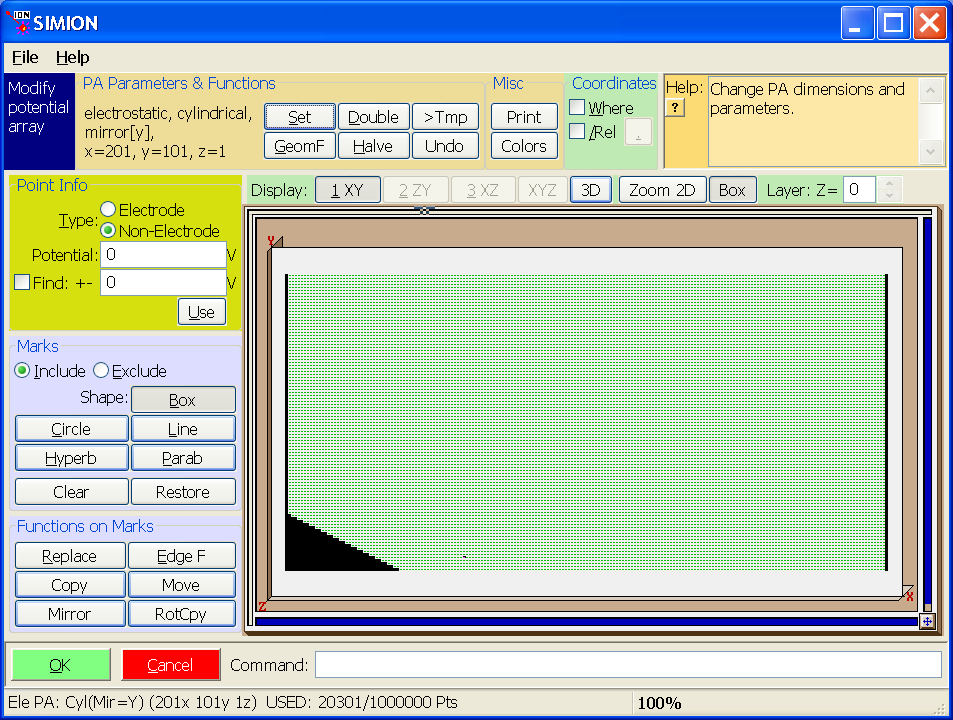
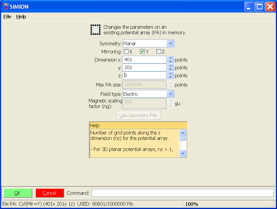
In SIMION, convert the point-big.gem to a potential array point-big.pa. It looks like this in Modify:

Refine point-big.pa (refined here to 1e-7 convergence) and go back into Modify.

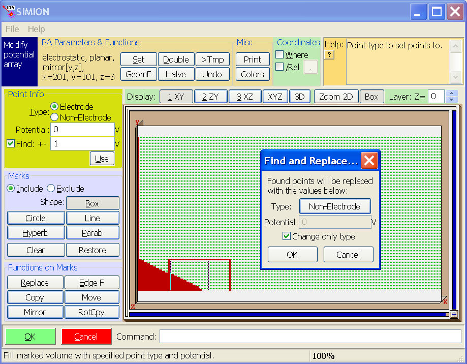
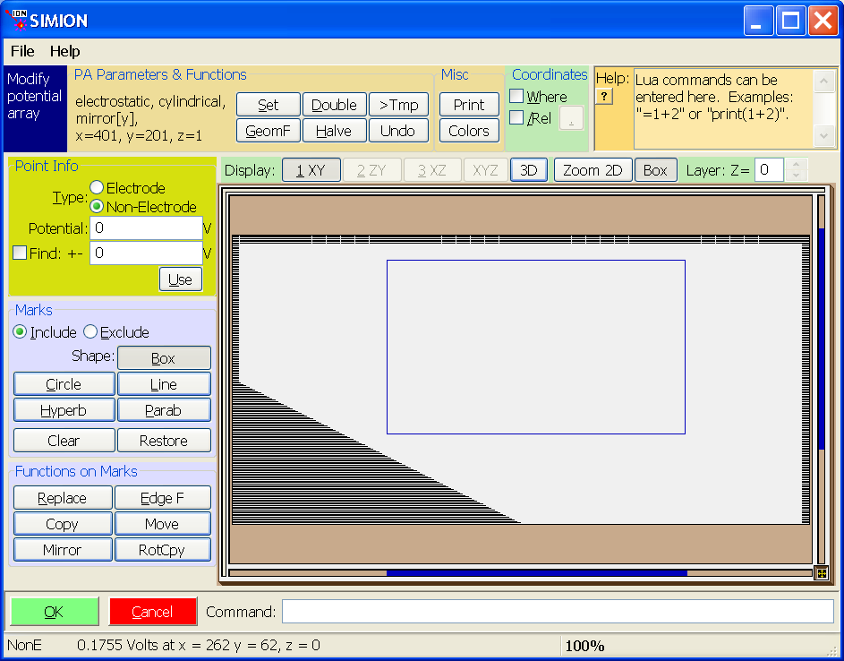
In point-big.pa, we want to convert the non-electrode points that will be on the boundary of the intersection of the two PAs to electrode points since View’s Copy function we will use only copies electrode points between arrays. Further, we want to convert any electrode points inside the intersection of the two PAs to non-electrode points (since we don’t want View’s Copy to copy any other points). We can do this in Modify by enabling the “Find” function with it set to find “Non-Electrode” points with Potential “0” V “+-” “1” V, marking a box around the boundary between the two PAs (i.e. from (x,y)=(20,0) to (x,y)=(60,20)), clicking “Edge F”, specifying “change only type” with “Type” set to “Non-Electrode”, and clicking “OK”.

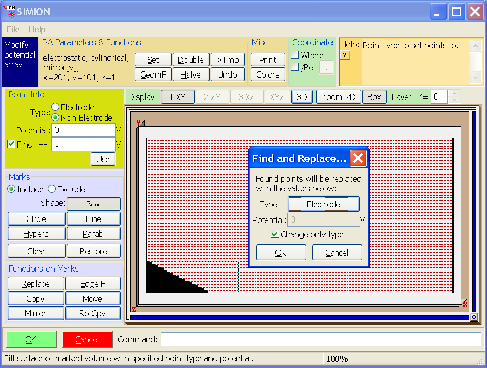
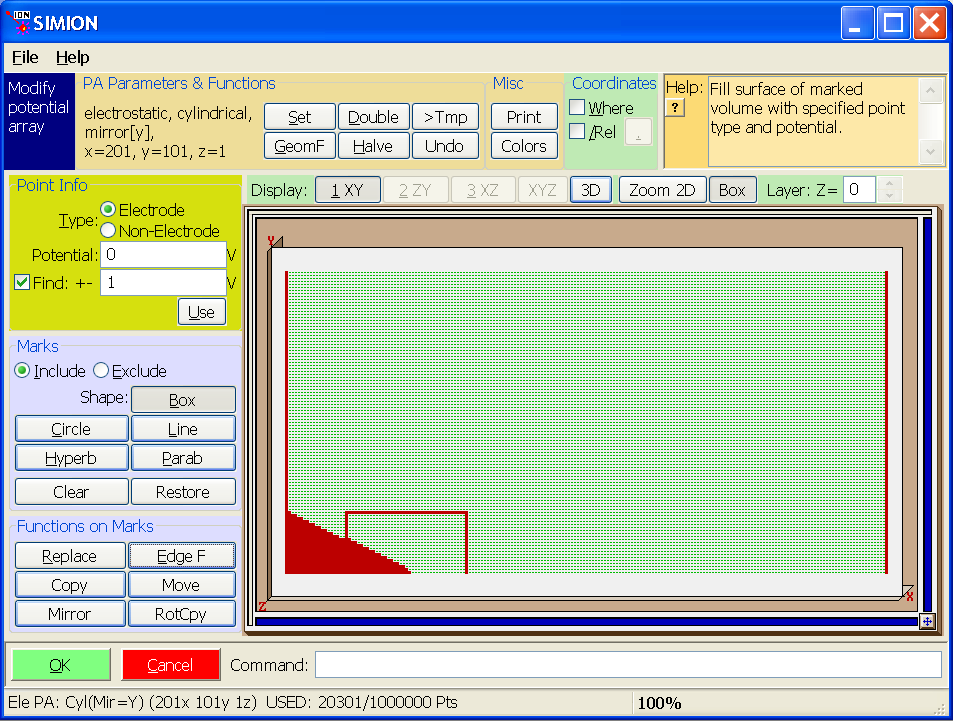
As shown below, the edge of this boundary box has been converted to electrode points. Importantly, the potentials on the box have the same potentials as the refined non-electrode points replaced:

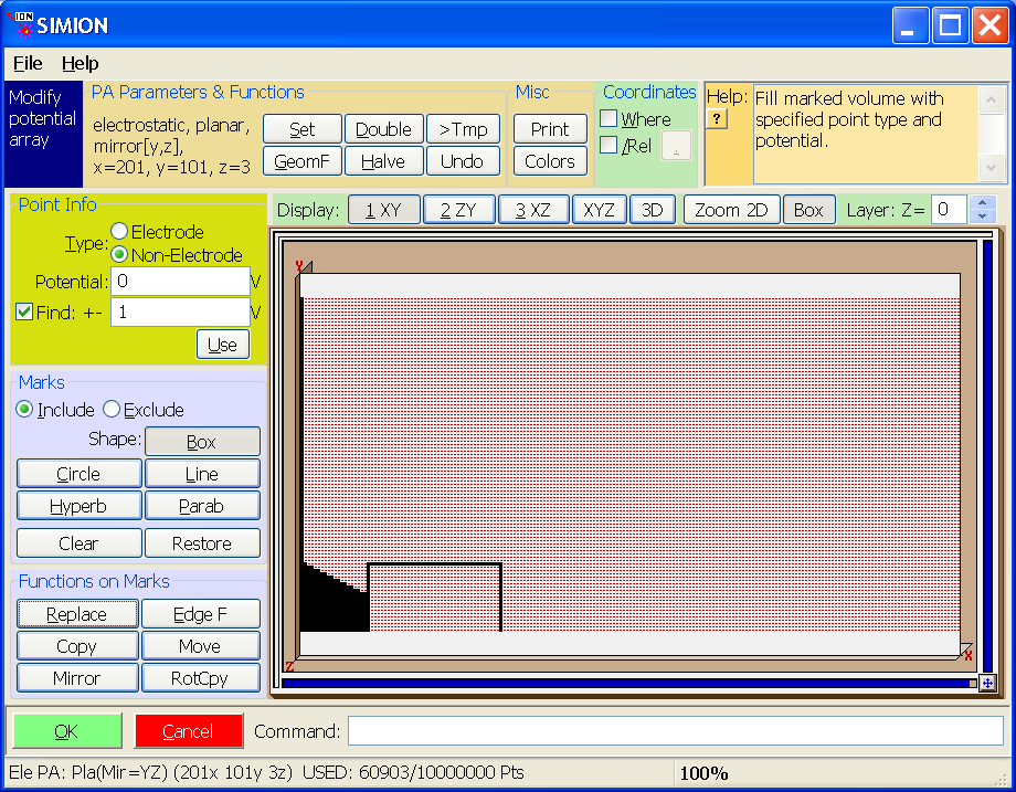
The next step is similar. Convert all points inside the box to non-electrode points (to prevent View’s Copy function from copying them). As before, we enable “change only type” this process (though it’s not as important here).

We see the result below. The location where the fine array will be placed is empty except for the electrode points on the boundary, which will be copied into the fine array.

Save the potential array.

Now, convert point-small.gem to a potential array point-small.pa. It looks like this in Modify:

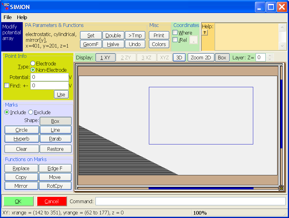
Save it.

Now, the following step is only required when using View’s Copy function to copy into a 2D potential array since the function currently (as of version 8.0.2) supports copying onto 3D potential arrays only. The trick is we use the “Set” function in Modify to temporarily convert both 2D point-small.pa and point-big.pa to 3D potential arrays (with z=3). Answer “Yes” to any questions. You may need to increase the “max PA size” on the main screen to 10 million points or so and reload the arrays so that there’s enough free allocated space to do this. Save both potential arrays.

Now View point-small.pa in View. Important: in general, do not refine if prompted to (our modified PAs might not refine correctly).

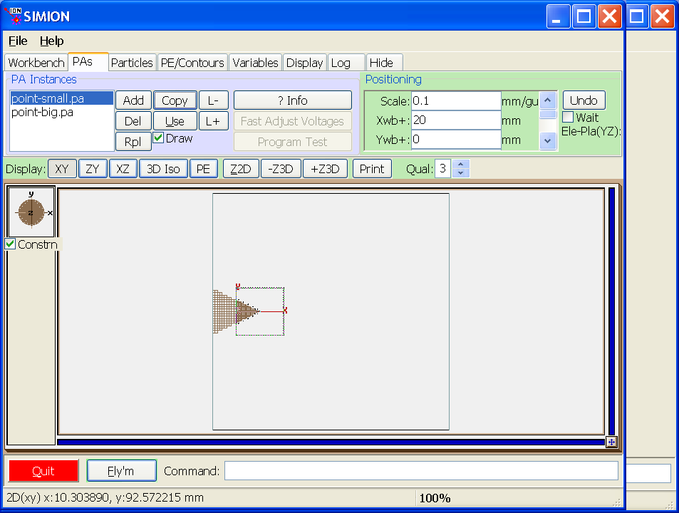
In the PAs tab, add the point-big.pa as well. Select the point-small.pa instance and set its scale to 0.1 and its Xwb+ to 20 so that the two potential array instance properly overlap. Notice that we have “point-small.pa” being the first instance in the list (for now at least), which is required since Copy points into the selected instance (point-small.pa) from instances listed after it (point-big.pa). Also, on the Workbench tab, you probably want to click “Min” to minimize the workbench size to tightly fit around your PA instances.

Now, with the point-small.pa selected in the PA instance list, click the “Copy” button. This copies electrode points from the later instances into the currently selected instance. Particularly, we are copying the calculated boundary conditions from the course PA into the fine PA.

At this time you may view point-small.pa in Modify to verify that the points were copied correct. (Note: the boundary is fairly thick–about 10 grid units. It would be a good idea to use Modify to cut the boundary back to 1 grid unit. The voltages across the boundary are also stepped every 10 grid units, which also would be best to improve (somehow).)

It’s important at this time to convert both PA’s back to 2D cylindrical using the “Set” function in Modify. Save both PAs.

Go back into View. (Note: there’s no need to rerefine if asked to, though it’s shouldn’t hurt in this case, but beware in general that the boundaries in your coarse array will still refine correctly after the modifications to it.)

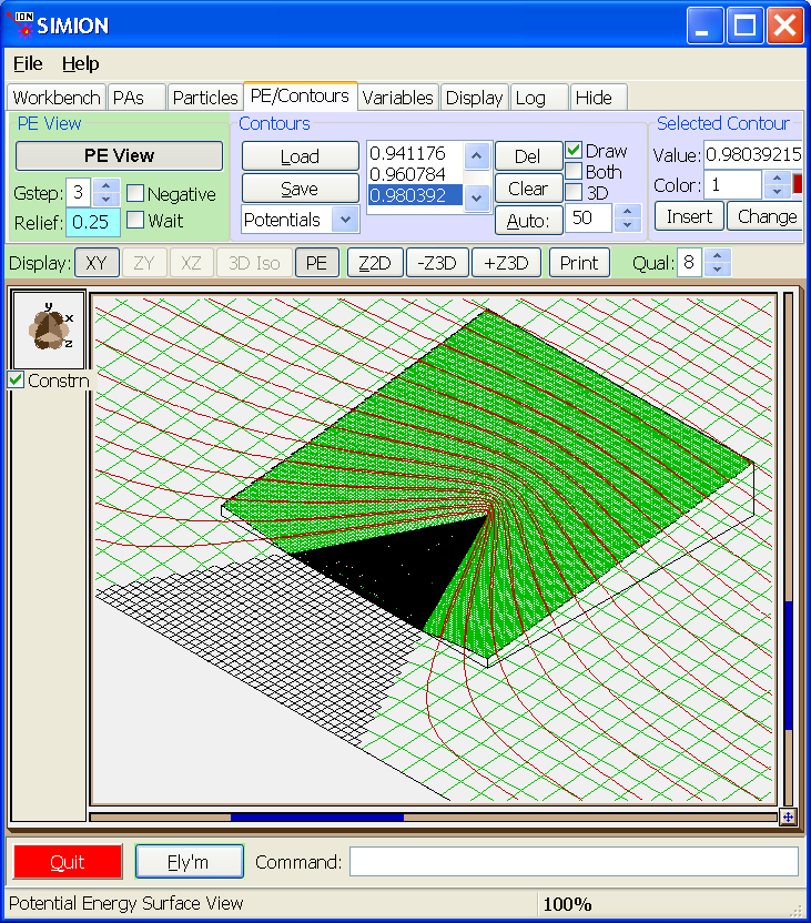
A potential energy view with contours is shown below. Note that the potentials generally match up on the boundary as required.

Before flying particles, switch the order of the two PA instances in the PAs tab (with PE view off, click “L-” with point-big.pa selected). This makes the course PA a lower priority than the fine PA. Particles flying inside the fine PA will see the (more precise) fields from the fine PA rather than from the coarse PA.


[Optional] Your name:	email:	phone: