Frequently Asked Questions (FAQ)
Installation
Which operating systems can SIMION run on? Are Mac OS and Linux supported?
SIMION is a native 32-bit or 64-bit Windows program that can run on all modern versions of Windows. SIMION is also formally supported under Linux via Wine and Mac OS X via CrossOver, provided your CPU is Intel x86 compatible (including x86-64), in which case SIMION runs at native speeds. Virtualization is another option though less seamless. If your CPU is not Intel x86 compatible (e.g. PowerPC, Sun MIPS, etc.), then you’ll likely have much less luck since an emulator would be required, which is undesirable on a heavy number crunching application like SIMION. For further details, System Requirements.
I’m a beginner. Where do I start learning to use SIMION?
Here’s some pointers:
For general background information on SIMION, see the six page SIMION 8.0 brochure.
Overview SIMION: Chapter 2 of the SIMION manual has a overview of SIMION and guides you through setting up a simple simulation. A copy of this chapter is also online.
Familiarize with the GUI: Appendix C “SIMION GUI” of the version 8 SIMION manual (Appendix F in SIMION 7) has a basic overview of the GUI. This is more important for the older version 7.
Explore examples: Appendix D “Sample Runs” of the version 8 SIMION manual (or Appendix C in SIMON 7) guides you through running a few of the examples. Once you know how to run examples, you can explore other examples in SIMION as well. Instructions are in the README.html files in each example.
A couple screencasts of SIMION operation can be viewed.
Chapters 3-8 of the manual describe in more detail the major components of SIMION. It can be useful to read this straight through, after getting a general overview of SIMION from the points above, but it can also be used as a reference.
See the SIMION Frequently Asked Questions (this file). For other specific topics see SIMION 2024 Supplemental Documentation.
The SIMION “short” and “advanced” courses may be of some help, though these are older (for version 7). These are in the “courses” folder inside SIMION’s program directory. Another SIMION-related course is at http://hipirms.org/ .
For any questions, ask us.
Already a user of a previous version?
New features in SIMION 8.1 are listed in SIMION® 8.1.
SIMION Advances - latest improvements in SIMION
Are SIMION 6.0/7.0 files compatible with 8.0/8.1?
Nearly all 7.0 (and 6.0) files will be used unmodified in SIMION 8.1 without any issue. Many SIMION 8.1 files can even be used on older versions, provided they don’t use new features added in those newer versions. Occasionally small differences occur such as due to some bug that is created or fixed, but that also affects minor version updates too and is rarely a showstopper. The full list of changes is at SIMION Software Change Log. Also, there can be minute differences in results since, for example, SIMION 8.1 uses CODATA2010 values of Physical Constants, but this is rarely an issue.
One minor difference from 6.0 is that for SIMION 6.0 PRG files, static variables used in initialize and terminate segments need to be changed to adjustable variables in SIMION 7.0 or above.
Features
How can I input geometries?
There are a variety of methods. See Geometry Input Methods.
Can collisional effects of ions flying through non-vacuum conditions be simulated?
See Ion-Gas Collisions.
Can space-charge effects be handled?
It has some capabilities for estimating the onset of space-charge. See Space Charge.
Can I write user programs in other languages?
SIMION version 8.0 supports Lua scripting, which is incorporated
into SIMION itself. It also supports calling code written in other
languages through the Lua interfaces (e.g. C/C++ can be compiled as
a DLL and called from Lua as shown in the “examples” example or by
compiling it as an EXE and running it via the os.execute or
io.popen Lua functions).
For compatibility, SIMION 8.0 also supports SIMION 7.0 PRG scripting,
which is a more primitive language.
You can of course also utilize any programming language (including Excel) to post-process SIMION data recording output files, build initial particle definitions (.ION files), or invoke SIMION commands via the batch mode interface.
Older notes (SIMION 7.0): Technically, SIMION 7.0 can only run PRG user programs, and there is no built-in extension mechanism for running other languages. However, the SL Toolkit add-on (since merged into SIMION 8.0) works around this in two ways, both within the bounds of PRG code. The first is to translate a high-level SL program into PRG code with the SL Compiler and then have SIMION run the PRG code. The second is to write an SL program that remotely communicates with a running C++ program (using the SL Remote libraries). SL Remote (use v.1.0.2 or above) achieves this essentially via remote procedure calls (implemented internally using some obscure, but largely hidden from the user, workarounds using named pipes pretending to be array files). The one downside is that remote procedure calls add some ~10x-100x time overhead if you’re doing thousands or millions of individual calls, one or more per each simulation time-step (rather than batching them). SIMION 8.0 avoids these complications.
How can a short movie of a SIMION simulation be created?
See Movie Files.
Using Features
How can the PA grid scaling be changed to other than 1 mm per grid unit?
See Scaling a PA.
How can I Change the Number of Points in a PA?
Use the Set button on the Modify screen to add more space
in a PA.
Use the Halve/Double buttons on the Modify screen scale down/up
the PA resolution (though this may lose accuracy compared to rescaling
a GEM or STL file and reconverting that to a PA).
The Set/Halve/Double buttons may impose a limit on number of points
you can add because the you can only resize the PA within the memory
block in RAM that the PA was loaded into.
To load the PA within a larger memory block:
Ensure the PA is saved to disk.
On the main screen, click
Remove All PAs from RAM.On the main screen, increase
Max PA Sizeto at least the number of points you will need in the new PA.Load the PA and resize using the Modify screen
Setbutton.
Why do Modify and View screen dimensions seem to differ by one grid point?
It is important to understand this distinction so that your electrode positions are not off by one grid unit.
The Modify function 2D views represent the points on the vertices of the grid cells. The electrode material fills the interior of those grid cells when the surrounding vertex points are marked as electrode points. The View screen and Modify 3D views visualize that actual electrode material. If in doubt, the View screen and Modify 3D views are what you should rely on for physical measurements.
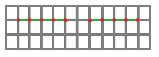
The following picture illustrates this. Each section of electrode plate (green) is defined by five grid points (red) but is of width 4 grid units and height 0 grid units (infinitely thin, 100% transmission ideal grid). The spacing between the two grid sections is 2 grid units. By default, each grid unit corresponds to 1 mm unless you change the mm/gu scaling factor (see above).
Consider also the below figures:
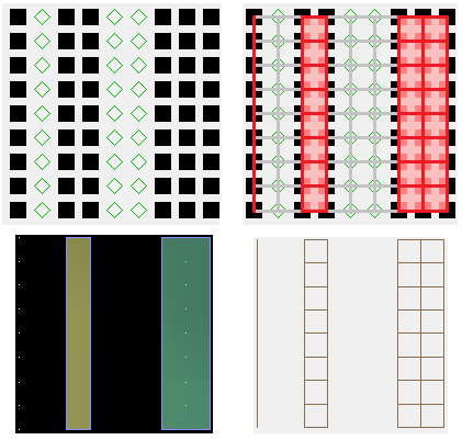
The top-left figure shows what some electrode points look like in Modify XY view. The top-right shows how those points are interpreted as electrode material (red). The bottom-left is the Modify 3D view, and the bottom-right is the View screen, both of which agree with the top-right figure.
Please note that Electrode Surface Enhancement / Fractional Grid Units complicates this. The Modify screen will display red bars where exact surface locations are. At the time of this writing (8.1.1.30), these red bars do not yet display on the Modify 3D or View screens though.
How can particle flight performance be increased? I want to disable screen redrawing and writing the large ion trajectory file (traj*.tmp).
In View, Particles tab, reduce the trajectory quality (T.Qual) from the default +3 to 0 (see the Computational Methods appendix of the printed user manual for details on the trajectory quality factor). Time-step sizes can also be controlled via user programs (tstep_adjust segments).
Disable data recording, or reduce the amount of data generated.
In View, Particles tab, uncheck the View box to disable displaying trajectories and uncheck the View box next to it to disable writing the traj*.tmp file (which stores trajectories for viewing purposes). In lieu of the traj*.tmp file, you can use the data recording or user programming features to more flexibly record only the data you need. The size of the trj*.tmp file is an additional concern on older file systems and libraries having a 4GB file size limit. If you do generate a trj*.tmp, make sure its on a fast disk (e.g. not a remote network share).
See also Calculation Time.
Older SIMION 7.0 Notes: In View, on the “Normal” tab, the “V” and “R” buttons control this.
I want to record the initial and final positions of a particle on the same line of an output file.
See Record the initial and final particle positions on the same line of an output file.
How can I Data Record periodically, such as for an FFT calculation?
See Data Record periodically, with constant size time steps, possibly for FFT.
What are PA/PA#/PA0/PA1/PA2/PA3 files? How do they differ?
How does the trajectory quality factor (T.Qual) relate to time-step sizes?
How can I force particles to stop at a certain location or time?
See Stop particles after given time or Stop particles at a certain location.
Can I suppress the “particles not created” warning?
The prompt “Warning: X of Y particles not created. Particle Z: terminated in electrode or beyond volume. Additional errors not displayed. Fly remaining particles anyway?” occurs if particles are created inside an electrode or outside the workbench volume. In such case, the particle will immediately terminate. Typical reasons for this are incorrectly defined particles (Particles Define screen) or statistical distributions in particle definitions that cause some fraction of the particles to be created in these regions. You can adjust the particle definitions to avoid this or just ignore this warning.
This message can prevent batch mode programs from running.
It can be suppressed by launching the Fly’m from the
command-line or SIMION command bar with the
--noprompt option:
simion.command '--noprompt fly c:/temp/drag-tmp1.iob'
How can a fast_adjust segment control electrodes in multiple arrays?
You can differentiate between PA instances using the
ion_instance reserved variable, which contains the sequence
number of the PA instance that the current particle is contained
in:
simion.workbench_program()
function segment.fast_adjust()
  if ion_instance == 1 then
    adj_elect01 = 20
    adj_elect02 = 30
  elseif ion_instance == 2 then
    adj_elect01 = 20
    adj_elect02 = sin(ion_time_of_flight)
  end
end
The above causes Electrodes 1 and 2 of the first PA instance to have potentials of 20 and 30 V respectively. In the second PA instance, Electrode 1 is set to 20 V and Electrode 2 is set to a sinusoidal waveform.
The way this works is that whenever SIMION wants to know the
electrode potentials, it sets various reserved variables (including
ion_instance) for the state of the particle it is currently
calculating, it calls the fast_adjust segment, and then it
reads the electrode voltages that the segment set.
The code can also be used in an init_p_values segment. The only
difference is that ion_instance takes a more general meaning
here: it is the “number of the PA instance that SIMION wants to
determine electrode potentials for”, making no mention about
particles since init_p_values is not called in the context of
particle flying but rather is typically is called before any
particles fly.
In a multiple-PA system, you may find simpler to not reuse
electrode numbers. In the above example, the second array could
instead have Electrodes 3 and 4. As of SIMION 8.0.4, PA# file
electrode numbers need not start at 1 nor be sequential
(Issue-I 414). However,
sharing electrode numbers is convenient if an electrode (e.g. #1)
spans multiple arrays, for then you can set the adj_elect01
variable regardless of PA instance number:
simion.workbench_program()
function segment.fast_adjust()
  adj_elect01 = 20  -- same regardless of ion_instance
  if     ion_instance == 1 then adj_elect02 = 30
  elseif ion_instance == 2 then adj_elect02 = sin(ion_time_of_flight) end
end
How can fast adjusting be prevented on IOB load?
Normally when save an .iob file, the current (i.e. in-memory) values of the .pa0/.pa array adjustable potentials are preserved in the .iob file. When you later re-load the .iob file, the .pa0/.pa arrays in memory will be automatically fast adjusted/scaled to the potentials previously saved in the .iob file. This may be undesirable particularly if you have some batch mode program that rebuilds the potential array files and then flies the existing .iob because the .iob will override any adjustable potentials in the potential array files with old values. It may also be unexpected when editing basic style .pa arrays, which get rescaled.
Disabling adjusting in batch mode: Here’s an example in batch mode to build .pa and .pa# arrays, refine them, fast adjust the .pa0, and fly an .iob containing both arrays:
simion.exe --nogui gem2pa one.gem one.pa
simion.exe --nogui gem2pa two.gem two.pa#
simion.exe --nogui refine one.pa
simion.exe --nogui refine two.pa#
simion.exe --nogui fastadj two.pa0 1=100,2=200
simion.exe --nogui fly test.iob
In the above example, upon loading (and flying) the .iob file,
the fast adjustments in the .pa0 file
(1=100,2=200) are ignored and the .pa may be rescaled.
You can prevent this using the --restore-potentials=0
option:
simion.exe --nogui fly --restore-potentials=0 test.iob
Omitting electrode potentials in .iob files:
In SIMION >= 8.1.1.21, upon saving an .iob file,
an option is presented to “save/retain” the “Electrode potentials (inside .iob),
to adjust PA potentials on .iob load”.
If you uncheck this box (by default it is checked),
then the electrode potentials are not preserved in the .iob file, so the PA’s will not
be fast adjusted/scaled upon .iob loading.
This is useful in GUI mode, and in batch mode it eliminates the need for the
fly --restore-potentials=0 option.
.iob files saved in this manner remain compatible and work as expected in
earlier versions of SIMION too.
Prompts to fast scale on .iob load:
SIMION >= 8.1.1.21 displays the prompt
“Fast scale these PA's in memory to match potentials from the IOB file?”
upon loading an IOB with a basic array (.pa) file whose scaling potential
does not match the scaling potential stored in the .iob file.
The default answer is Yes, but you should choose No if the PA file is correct and should not be rescaled.
(To avoid this prompt in the future, resave the PA file and/or IOB file to ensure consistency.
A simple way to save both is to ensure “saving/retain” of both “Potential arrays (.pa/.pa0)”
and “Electrode potentials (inside .iob)” when saving the .iob file.
Alternately, force a No by disabling “saving/retaining” of
“Electrode potentials` (inside .iob)” when saving the IOB file.
An answer can also be forced in batch mode via the fly --restore-potentials=0,
fly --restore-potentials=1 or --noprompt options.)
This prompt is intended to avoid unintentional rescaling of .pa files after editing
.pa files and reloading the .iob.
This prompt does not occur for fast adjustable array (.pa0) files though.
A similar prompt existed in SIMION 7.0
(”Restore Potentials To Values Active When .IOB Was Saved?”)
but was removed in SIMION 8.0 to reduce excessive nagging.
This prompt has been re-added except it now only displays much less frequently
and it is more informative.
How can a custom distribution be added to a FLY2 file?
See “Custom Distributions in FLY2 files” in FLY2 File.
What is CWF in the particle definitions?
CWF is the charge weighting factor. It’s used particularly by SIMION for the charge repulsion feature (detailed in SIMION Example: repulsion and in the Calculation Methods appendix of the SIMION User Manual, but see also Space Charge for other approaches). If charge repulsion is disabled (as it usually is), SIMION ignores this field, and it is typically left at its default value of 1 though you could store whatever you want in it (e.g. see Monte Carlo Method). Each particle simulated in SIMION often represents a certain amount of real physical particles in your system. The CWF allows so you say that some simulated particles represent more physical particles than others. If you set CWF to the same value for all particles (e.g. the default 1), then all simulated particles are weighted identically.
In CAD import (STL to PA), all electrodes are set to 1V.
How can I import or export field or PA data?
How can I combine electric and magnetic fields?
Errors
My PA contains a single electrode, but no fields are shown.
In short, in order for a non-zero field to be calculated inside a PA, the PA must contain at least two electrodes of dissimilar potentials. All space potentials computed inside the array will be bounded between the minimum and maximum electrode potentials. Furthermore, if you have two electrodes and you place each in a separate PA, this will not work either because fields in each PA are normally solved independently.
The underlying reason for this is rooted in the properties of the Laplace Equation, upon which the SIMION field solver (Refine) is based. The Laplace equation can be uniquely solved only if suitable boundary conditions are specified over some surface enclosing the volume containing your field. Points with known potential, such as electrode surfaces, define one type of boundary conditions (Dirichlet Boundary Conditions). If the boundary points on your PA are not electrode points, SIMION assumes, for lack of better direction from the user, that these points have Neumann Boundary Condition) (derivative of potential along the direction normal to the boundary surface is zero). Neumann conditions are required over mirror symmetry planes wherever Dirichlet conditions are lacking. A sure way to obtain a reliable field is to place all your electrodes plus an enclosing Ground Chamber electrode in a single PA.
See First Uniqueness Theorem for more details.
When I fast adjust my potential array, it only shows a single electrode #0
If you need to fast adjust electrodes potentials individually and independently,
you need to save your potential array with a .PA# not .PA file name extension.
A .PA file is just a basic potential array; all electrode potentials can be
rescaled by the same proportion but not adjusted individually and independently unless
you refine the whole array again.
In contrast, a .PA# file is a fast adjust definition array, which upon refining generates a
fast adjust base solution array (.PA0), which has additional solution arrays
(.PA1/.PA2/etc. files) for each electrode to allow
the electrode potentials to be independently “fast” adjusted without refining again.
Also, the .PA# file should contain positive integer electrode numbers (1, 2, 3, etc.)
not actual voltages, unless you don’t want them to be adjustable.
Voltages are defined later (after Refine) in the .PA0 file by Fast Adjust.
A discussion of .PA and .PA# file differences is in Potential Array File Types (Comparison).
My PA has nz=1 and no symmetry, but in ISO View it looks like a brick 100 units thick.
A PA with nz=1 (i.e. one grid point, or zero width, in the Z dimension) is treated specially by SIMION as a system with 2D planar symmetry with the geometry in the XY plane projected infinitely down the z axis. When the array is placed into a workbench, you can limit the extent of this z projection to a finite value (SIMION 8.0: View screen, PAs tab, Positioning panel, “nz use” field in grid units) (SIMION 7.0: Ion Optics Workbench | PAs | Edit | nz use” field). The “examples.pa#” array is an example of this, which represents a 2D cross-section of infinitely long rods.
You may have an electrode like a metal plate or a wire mesh that might itself be representable on a 2D plane, and you might be tempted to model it using a 2D PA. However, the field in-front or in-back of the plate likely lacks 2D symmetry, so you need a 3D array to represent this field. Using a 3D array with the smallest number of points in the Z direction (e.g. nz=2) is still insufficient: You must include sufficient extra space and other electrical conductors facing the plate inside the array in order for the SIMION Refine function (Laplace solver) to properly calculate and represent the fields in the regions facing the plate. See Grid and First Uniqueness Theorem for further details on this.
My user program is not being called
Some things to check:
Does your Lua user program have the same name as your IOB file except with extension
.lua? For example, in SIMION Example: drag, the filesdrag.luaanddrag.iobare in the same folder and they have the same base file name (drag). SIMION will only use your user program if you give it the name it expects. (If you are using older SIMION 7.0 .prg programs, the .prg files must match the names of the PA’s not the IOB’s.)If you click the “User Program…” button on the Particles tab (in SIMION 8.0/8.1), does it display your user program? If no, then your user programs are probably misnamed (see previous point). (Note that prior to SIMION 8.1.0.45, this button only opens Lua programs not older SIMION 7.0 style PRG programs.)
If your user program contains adjustable variables, are they displayed in the Variables tab? If not, then your user program is not found, can’t be compiled, or contains no adjustable variables.
Is the “Use program” checkbox checked on the Particles tab? It should be.
Is any error message displayed when you click Fly’m? If yes, what is that error? Such an error may indicate that SIMION found and tried to call your user program but found an error in it (and you would not get that error if you removed your user program file). The error message should explain what is wrong, including the line number in your program where the error occurs.
If the user program is loaded but only the
initializeorterminatesegments are not being called, make sure your particles are inside the volume of a PA instance as described in My initialize and terminate user programming segments are not executed..
My initialize and terminate user programming segments are not executed.
Some segments might not be called when a particle is a particle is inside
a workbench volume but outside all PA instance volumes.
For example, initialize and terminate are normally called
each time a particle is respectively created or terminated inside
the volume of a potential array instance (sometimes excluding boundaries).
When a particle is inside both electric and magnetic PA instances,
these segments are called twice per particle inside.
This holds true for most segment types: segments
only execute within the context of particles and potential array instances,
and you can use code like this to only perform an action for a certain
PA instance or particle number:
function segment.terminate()
  if ion_instance == 1 and ion_number == 1 then
    print(ion_number, ion_px_mm)
  end
end
In SIMION 8.2-EA20170210, there is a new reserved variable
sim_segment_global which will cause segments to be executed
exactly once when particles are outside PA instance volumes, which may be
more like you want.
For earlier SIMION versions, you will need to use other approaches discussed
later.
simion.workbench_program()
sim_segment_global = 1  -- call segments everywhere
function segment.terminate()
  if ion_instance == 1 and ion_number == 1 then
    print(ion_number, ion_px_mm)
  end
end
But even that might not be desired.
terminate may be called once per particle, any you may have
zero, one, or multiple particles.
But what if you want to ensure something is done exactly once
at the end of the run?
SIMION 8.1.0.32 adds new segment.initialize_run()
and segment.terminate_run() segments that are called exactly once
per run regardless.
These new segments are simpler and more robust
for executing code that must be called exactly once before and/or after each run.
(The initialize/terminate segments, however, remain convenient for accessing particle
parameters because these segments gain read/write access to data on each particle
and PA instance via reserved variables.)
simion.workbench_program()
sim_segment_global = 1  -- call segments everywhere
local max_x = -math.huge
function segment.terminate()
  if ion_instance == 1 then
    max_x = math.max(max_x, ion_px_mm)
  end
end
function segment.terminate_run()
  -- this is called exactly once.
  print('max x=', max_x)
end
In SIMION versions prior to 8.1.0.32, you can, with care, achieve an effect similar to these new segments using techniques like this:
simion.workbench_program()
function segment.initialize()
    if ion_instance == 1 and ion_number == 1 then
        print 'this should execute once'
    end
    -- warning: This SIMION 8.0 workaround fails if particle #1 is
    --          not created inside PA instance #1.
end
If you need to ensure initialize/terminate segments are always
called once for SIMION versions prior to 8.2 EA 20170210,
there are some other techniques you can use.
First, just take care in defining your particle starting points and
make sure your particles don’t exit your potential arrays and then
splat outside.
Clicking the “Min” button on the Workbench tab will
shrink your workbench volume to more tightly surround your
potential arrays and may eliminate dead-volume.
You may need to force your particles to terminate inside the array volume.
For example, a user program to keep ions approximately within a certain
box volume can look like this:
simion.workbench_program()
function segment.other_actions()
   if not(ion_px_mm > 10 and ion_px_mm < 20 and
          ion_py_mm > 10 and ion_py_mm < 20 and
          ion_pz_mm > 10 and ion_pz_mm < 20)
   then
       ion_splat = 1
   end
end
Alternately, you may add electrodes, or an entire ground cage, that act as stoppers. Extra electrodes do affect fields, but you can avoid this by creating a larger array of solid electrode points that contains your real array but is at a lower priority number in the PAs tab PA Instances list, in which case the particles only see the larger array if they exit the smaller array, and on entering the larger array they will immediately splat.
To confirm whether initialize and terminate segments are being
called, you may add print statements in a user program:
simion.workbench_program()
function segment.initialize()
    print('initialize', ion_instance, ion_number)
end
function segment.terminate()
    print('terminate', ion_instance, ion_number)
end
fast_adjust segment behaves oddly with Grouped flying enabled or ion_time_of_flight reverses direction
fast_adjust segments should be written carefully to avoid them being
dependent upon a certain order of execution. SIMION is free to call
fast_adjust segments in any order, so wrongly assuming a particular
order may lead to situations where a fast_adjust segment seemingly
works in one situation but fails in another.
To see this, note that the user program
simion.workbench_program()
function segment.fast_adjust()
  print(ion_number, ion_time_of_flight)
end
function segment.other_actions()
  print('*')
end
with two particles might print results like
1 0.000   1 0.000   1 0.025   1 0.025   1 0.050   1 0.000   *
1 0.050   1 0.075   1 0.075   1 0.101   1 0.050   *
1 0.101   1 0.126   1 0.126   1 0.151   1 0.101   *
...
2 0.000   2 0.000   2 0.025   2 0.025   2 0.050   2 0.000   *
2 0.050   2 0.075   2 0.075   2 0.101   2 0.050   *
2 0.101   2 0.126   2 0.126   2 0.151   2 0.101   *
...
and with Group mode flying enabled might print results like
1 0.000   2 0.000   1 0.000   1 0.025   1 0.025   1 0.050
 1 0.000   2 0.000   2 0.025   2 0.025   2 0.050   2 0.000   *   *
1 0.050   1 0.075   1 0.075   1 0.101   1 0.050   2 0.050
 2 0.075   2 0.075   2 0.101   2 0.050   *   *
1 0.101   1 0.126   1 0.126   1 0.151   1 0.101   2 0.101
 2 0.126   2 0.126   2 0.151   2 0.101   *   *
...
and with overlapping magnetic and electric PAs, you might see twice
the number of ‘*’ markers, and if sim_update_pe_surface = 1 is
further added to the other_actions segment with PE viewing enabled, you might see
results like this:
1 0.000   2 0.000   1 0.000   1 0.025   1 0.025   1 0.050   1 0.000
 2 0.000   2 0.025   2 0.025   2 0.050   2 0.000   *   1 0.000   *   *  2 0.000   *
1 0.050   1 0.075   1 0.075   1 0.101   1 0.050   2 0.050   2 0.075
 2 0.075   2 0.101   2 0.050   *   1 0.050   *   *   2 0.050   *
1 0.101   1 0.126   1 0.126   1 0.151   1 0.101   2 0.101   2 0.126
 2 0.126   2 0.151   2 0.101   *   1 0.101   *   *   2 0.101   *
...
As seen, the order in which fast_adjust segments are executed is
not always obvious. The ‘*’ markers above indicate that the
fast_adjust segment is evaluated multiple times per time-step per
particle. Typically it evaluates five times, though sometimes it is
more or less, such as when approaching boundaries. Within each
time-step, the fast adjust times are not entirely in chronological
order, particularly on the fifth and sometimes later evaluations.
When flying ions individually (Grouped checkbox disabled), each time a
new particle trace is started the time is reset to the current
particle’s time-of-birth (typically zero). When Grouped mode is
enabled, the fast adjustments in each time step are evaluated
concurrently for all flying particles. When reruns are enabled, the
time is reset to zero upon the start of each rerun. In other
occasions, like with sim_update_pe_surface set, additional
fast_adjust calls may be made. See also the updated flow diagram
(Issue-I 304) to further understand the behavior.
The lesson learned from this is that you should not rely on the
fast_adjust segment being executed in any particular order. The
fast_adjust segment should make its voltage adjustments using only
the information in the reserved variables passed to it, such as
ion_time_of_flight, ion_number, ion_instance, etc. It
should not make its adjustments based on “side-effects” from other
variables external to the current invocation of the fast_adjust
function. For example, to define a square waveform, don’t do something
like this:
-- bad
simion.workbench_program()
local offset = 0  -- state external to the function call
function segment.fast_adjust()
  if ion_time_of_flight - offset > 3 then
    adj_elect01 = -10
    if ion_time_of_flight - offset > 10 then
      offset = offset + 10 -- warning! modifies external state
    end
  else
    adj_elect01 = 10
  end
end
The effect of this segment depends on the previous value of
offset, which in turn depends on how the segment was previously
called. Write it instead like this:
-- good
simion.workbench_program()
function segment.fast_adjust()
  local fraction = ion_time_of_flight % 10
  local Vmax = ion_number * 10
  if fraction < 3 then
    adj_elect01 = Vmax
  else
    adj_elect01 = -Vmax
  end
end
Not only is this second version more correct, but it is also easier
to understand. Its behavior in how it sets adj_elect01 depends
solely on the current values of ion_time_of_flight and
ion_number (even if time reverses in direction or is random).
If you need to write logic that depends on strictly increasing
time, put this logic in an other_actions segment instead, and
if necessary reset any state prior to flying new particles or
starting new reruns. Enable Grouped flying on the Particles tab is
you want all particles to fly simultaneously rather than one after
the other.
See also Time.
“Failed saving PA file: Access is denied” error on refining or flying in Windows Vista/7
Windows Vista/7/8 file permissions by default do not allow standard (non-administrator)
users to save or modify files in the c:\Program Files (or c:\Program Files (x86))
folder. If you attempt to refine or fly examples contained in these folders
(e.g. under c:\Program Files\SIMION-8.1\examples), you
may receive an error such as Failed saving PA file: Access is denied or
The operating system is not allowing you to write the file.
It is recommended to copy the example folders to some personal location
where you have full permissions (e.g. your
desktop or My Documents folder) prior to running them in SIMION.
This approach is recommended over
simply granting yourself permissions to the c:\Program Files\SIMION-8.1\examples
folder because it preserves a copy of the original versions in case you ever want to
go back to them, and it is also more secure on a multi-user system.
Refining PA# arrays, flying with trajectory retaining enabled, or using Data Recording with an output file are a few cases where SIMION may attempt to write files to the same directory.
Errors - SIMION 7.0
Fails to install SIMION 7.0 on a 64-bit system
SIMION 7.0 is a 32-bit program, which runs fine on 64-bit Windows. However, the installer for SIMION 7.0 was 16-bit, which 64-bit Windows can’t run. The workaround is to install SIMION 7.0 on a 32-bit system, copy the program folder to your 64-bit system, and then uninstall it from your 32-bit system.
I get the error “Directories Missing: More than a Total of 3000 in Drive” or “Directory File Too Big to Totally Load” error in File Manager or don’t see all directories…
This issue affects version 7.0. It it is fully resolved in version 8.0, which replaces the GUI File Manager with a regular Windows File Open dialog box. This issue is somewhat resolved in version 7.0.2 and later, which improves the GUI File Manager a few ways. We recommend SIMION 7.0.0 users download the free upgrade to the latest 7.0.x version’’’ to mitigate this problem.
In version 7.0.0, there were three known workarounds, which we no longer generally recommend but still provide here mainly for historical reference. The resolution incorporated into 7.0.3 is effectively similar to Solution #1 below but is simpler and does not do an actual drive mapping.
Old Solution #1 - Download and save the simion.bat program file. Add this file to your start menu or desktop. Now, always start SIMION by double clicking this simion.bat program rather than the regular SIMION program icon. Notes: If your system does not have an unused “S:” disk drive letter or your SIMION program directory is not “c:7”, then simion.bat should fail. To correct this, you will have to edit the simion.bat file to set these these two variables to values compatible with your particular system configuration. Technical details: simion.bat is merely a wrapper around the standard SIMION program (simion.exe) and creates a “virtual drive” for the SIMION program folder using the DOS command “subst S: c:7”). When SIMION’s GUI file manager then starts up, it will only scan the files in this virtual drive rather than all files on your main hard disk. (tested on Windows NT and XP).
Old Solution #2: Rename any directory you need to access from SIMION by prepending and underscore (”_”) character to it. For example, you might rename the Sim7 directory to _Sim7. The directory should then be visible, but the error will still display.
Old Solution #3: Put all your SIMION related files on separate disk drive or partition that has fewer files (if you do have such a drive or partition). Alternately, create a “virtual” drive by creating a Windows network share on your SIMION directory and then assigning that share a drive letter (which is what solution #1 above does). Then access your files in SIMION from that drive letter. This can also be done via “Tools | Map Network Drive” in Windows Explorer.
“Initializing Random Number Generator” is displayed and program freezes with CPU at 100% during SIMION 7.0 startup.
This issue affects SIMION 7.0.0 to 7.0.2. It is fixed in version 7.0.3. We recommend you download and install the latest 7.0.x version of simion.exe, which is a free upgrade from 7.0.0.
This error happens in 7.0.0 if the system is not rebooted for ~24 days or more. If you have updated 7.0.0, a quick fix is to simply reboot your system. Another solution in 7.0.0 has been to disable the re-initialization of SIMION’s random number generator (p. E-15 of the SIMION 7.0 manual).
Viewing
Can I change the coordinate system so that particles move along Z rather than X?
A convention in SIMION is that electrodes with 2D planar or 2D cylindrical (i.e. axially symmetric) symmetry are drawn onto a 2D array mapped to the XY plane, where X is the axis of symmetry in the 2D cylindrical case. Therefore, the general direction of a particle beam though a cylindrical lens would normally be defined as the X axis. 3D arrays don’t have such restrictions, but the initial view for the array still defaults to displaying the XY plane, so the same preference for the X axis is often kept.
You can, however, orient arrays and particles however you want into a workbench, so
you are not limited to the above convention.
You could, for example, position a 2D cylindrical array into a workbench
such that the axis of rotation in the array (x) is aligned to the Z axis in the
workbench. This is done via “View > PAs > Positioning > Rotation” (in SIMION 8.0/8.1).
Your particle definitions can be defined relative to either the PA coordinates or to these
(rotated) workbench coordinates (“View > Particles > Define… > Coordinates relative to”).
Likewise, the coordinates displayed on the View screen are normally in these workbench
coordinates (“View > Display > Location > mm”), as are Data Recording output
and many programming variables (ion_px_mm). You can rotate the view to whichever plane
you want via the XY, ZY, XZ, or 3D Iso buttons or by dragging the “globe”. Therefore,
if you prefer particle beams to be aligned to the Z axis and analyzed as such, you can do so.
Note also: when using GEM files, some commands have a preference for a certain axis, but
you can also surround these commands with a locate statement that does a rotation.
Other
How do I run Lua code in SIMION?
How do I disable relativistic effects?
My changes to adjustable variables are ignored.
How can I make markers different colors, like when particles hit electrodes or test planes?
Set the marker color on the View screen Particles tab to 15. The value 15 (transparent) takes special meaning: it tells SIMION to use the same color for the marker as for the particle. Particles in turn can be colored individually via the Define Particles screen. (Note: Prior to SIMION 8.0.7-TEST8, you may need to temporarily enable time markers on the View screen Particles tab to change the marker color.)
Additional Notes
For additional topics, see SIMION 2024 Supplemental Documentation.
Is something missing from this FAQ? Questions or requests for clarification are most welcome.