ASMS Short Course on SIMION¶

Ion Optics Through the Eyes of SIMION - An ASMS Short Source

Portland ASMS Conference, May 11-12, 1996, Instructors: David A. Dahl and Anthony D. Appelhans

These notes were originally developed for SIMION 6.0. They are being updated to the latest SIMION 8.x version (in progress):

sessions 1-6 - updated to SIMION 8.x
sessions 7-10 - SIMION 6 (not updated)

Session 1 - Learn GUI/SIMION Usage ¶

Section 1 - Lab on Learning GUI/SIMION Usage ¶

This Lab’s Files are found in Directory: courses\short\session1 .

Learn by doing Discussion (SIMION main menu visible):

- GUI Objects (buttons, windows, etc.)
- Use Load (load EXTRACT.PA into memory)
- Enter View (demonstrate view orientations and drawing quality options). Say Yes if prompted to Refine and then click Refine.
- Class Activity (Load EXTRACT.PA and change view orientation and drawing quality)
- Demonstrate 2D Zoom and Scrolling via area marking
- Demonstrate 2D Zoom and Scrolling via Window button (both page and normal view)
- Class Activity (Practice 2D Zooming and Scrolling)
- Introduce 3D Zoom Volumes
- Demonstrate 3D Zoom via area marking
- Demonstrate 3D Zoom via the Window Button (page and normal view) and within-view pointing
- Class Activity (Practice the various forms of 3D Zooming)
- Remove all .PAs from memory
- Load EINZEL.IOB demo into View
- Load the EINZEL.FLY2 file (from the Define Particles button on the Particles tab).
- Fly ions (alone, grouped, as lines, and dots)
- Class Activity (Load EINZEL.IOB, EINZEL.FLY2, and fly ions in various ways)
- Demonstrate Potential Energy Surfaces
- Demonstrate Contouring (2D and 3D)
- Class Activity (Exercise PE surface and contouring options)
- Demonstrate use of Rerun and how to single time-step ions
- Demonstrate use of Fast Adjust while Ions are Flying
- Class Activity (Exercise Fast Adjust and single time-step options while ions are flying)
- Discuss/Demonstrate charge repulsion (Factor - beam)
- Class Activity (Practice using beam repulsion with EINZEL)
- Discuss how to print (view, objects, or entire screens)
- Introduce the various printing options
- Discuss how to use the annotator
- Class Activity (Print a selected view and an entire screen)

Session 2 - Ion Optics Concepts ¶

Some Basic Ion Optics Concepts ¶

Equations From Basic Physics:

$Force = Mass \cdot Acceleration$

$F = M A$

$Work = Force \cdot Distance$

$Force_{avg} = Work / Distance$

$F = dW/dr$

Coulomb’s Law:

$F_e = k Q_i Q / r^2 \textrm{ Point charge}$

$F_e = Q_i Sum_n (k Q_n / r_n ^ 2) \textrm{ Point charges}$

$Q_i = \textrm{The Ion's Charge}$

$E = F_e / Q_i = d(W/Q_i) / dr \textrm{ Electric field intensity}$

$E = Volts / Meter$

$Volts = Joules / Coulomb$

$F_e = -e E \textrm{e = units of positive charge}$

Electrostatic Equation of Motion:

$A = F / M$

$A = dv / dt = - (e E) / m = - E / (m / e)$

Magnetic Force Equation:

$F_m = Q_i (U X B) \textrm{Vector Cross Product}$

$Q_i = \textrm{The Ion's Charge}$

$U = \textrm{Vector Velocity of Ion}$

$B = \textrm{Vector Magnetic Field Intensity}$

Magnetic force is always normal to both the B magnetic field vector and the U velocity component normal to the B magnetic field vector (following the right hand rule):

$U X B = (U_y B_z - U_z B_y) i_x + (U_z B_x - U_x B_z) i_y + (U_x B_y - U_y B_x) i_z$

A simpler equation results from using only the vector velocity component normal to the magnetic field:

$F_m = Q_i U_n B (F_m \textrm{normal to both} U_n \textrm{and} B)$

$U_n = \textrm{Velocity component normal to B}$

Static Magnetic Equation of Motion:

$A_n = F / M$

$A_n = (dv/dt)_n = (e U_n B) / m = U_n B / (m / e)$

Note: Static magnetic fields change an ion’s direction of motion but not its speed (kinetic energy).

Refraction in Ion Optics ¶

Refraction (bending of ion trajectories) results from electrostatic and/or magnetic forces normal (at 90 degrees) to the ion’s velocity.

The Electrostatic Radius of Refraction

$\textrm{Normal Electrostatic Force = Centripetal Acceleration}$

$- e En = m v^2 / r_n$

$r_n = m v^2 / (- e E_n) = -(m/e) v^2 / E_n = -2 KE / (e E_n)$

$\textrm{where} KE = m v^2 / 2$

The Magnetic Radius of Refraction

$\textrm{Normal Magnetic Force = Centripetal Acceleration}$

$B_n e v = m v^2 / r_n$

$r_n = m v / (B_n e) = (m/e) v / B_n = (2 m KE)^(1/2) / (e B_n)$

$\textrm{where} KE = m v^2 / 2$

Interpretations of Radius of Refraction:

1. The electrostatic radius of refraction is proportional to the ion’s kinetic energy per unit charge. Thus all ions with the same starting location, direction, and kinetic energy per unit charge will have identical trajectories in electrostatic (only) fields. Trajectories are not mass dependent in electrostatic fields.

2. The magnetic radius of refraction is proportional to the ion’s momentum per unit charge. Thus all ions with the same starting location, direction, and momentum per unit charge will have the identical trajectories in static magnetic (only) fields. Trajectories are mass dependent in static magnetic fields.

3. Because of the v verses v2 effects on the radius of refraction, magnetic ion lenses have superior refractive power at high ion velocities.

Light Optics Verses Ion Optics ¶

There are significant differences between light and ion optics:

Radius of Refraction

Light optics make use of sharp transitions of light velocity (e.g. lens edges) to refract light. These are very sharp and well defined (by lens shape) transitions. The radius of refraction is infinite everywhere (straight lines) except at transition boundaries where it approaches zero (sharp bends). Ion optics makes use of electric field intensity and charged particle motion in magnetic fields to refract ion trajectories. This is a distributed effect resulting in gradual changes in the radius of refraction. Desired electrostatic/magnetic field shapes are much harder to determine and create since they result from complex interactions of electrode/pole shapes, spacing, potentials and can be modified significantly by space charge.

Energy (Chromatic) Spreads

Visible light varies in energy by less than a factor of two. Ions can vary in initial relative energies (or momentum for magnetic) by orders of magnitude. This is why strong initial accelerations are often applied to ions to reduce the relative energy spread.

Physical Modeling

Light optics can be modeled using physical optics benches (interior beam shapes can be seen with smoke, screens, or sensors).

Ion optics hardware is generally internally inaccessible and must normally be evaluated via end to end measurements. Numerical simulation programs like SIMION allow the user to create a virtual ion optics bench and look inside much like physical light optics benches.

Session 2 - Lab on Radius of Refraction ¶

Flying ions in a Cylindrical ESA

This Lab’s Files are found in Directory: courses\short\session2

Remove All PAs From RAM
Use View Function to load LOWELECT.IOB (cylindrical ESA)
Click the Define Particles button on the PAs tab (to access the particle definitions screen) and load 2LOWKE.FLY2 ion family file (two 100 eV ions: 100 amu - red, 1,000 amu blue). Click OK to return to the View screen.
Click the Data Recording button on the PAs tab to access the Data Recording Screen. Load the RECORD.REC data recording definition file. Ensure the Record check box is checked to turn data recording on. Click OK to return to the View Screen.
Click Fly’m button to fly the ions. Write down the time-of-flight (TOF).
Fly the ions grouped as dots and watch.

Notice that both ions have the same trajectory, although their velocities and time-of-flight (TOF) are different (ion trajectories in electrostatic fields are KE not mass dependent). Verify that the changes in TOF relate to changes in ion mass.

Changing Ion KE and electrostatic field strength

Click PAs tab and then Fast Adjust Voltages button and write down the electrostatic potential.
Change Potential (play a bit), re-fly the ions and look at the results. (ReRun can be used for movies.)
Change ion’s energies (in the Define Particles screen), re-fly the ions and look at the results.

Compensating for Increasing Ion KE within an electrostatic field

Use Load button within View Screen Workbench tab (not from Main Menu Screen) to load the HIELECT.IOB file.
We have increased the electrostatic field (via HIELECT.IOB). Now we need to load and fly higher energy ions. Click the Define button (to access Ion Definition Screen) and load 2HIGHKE.FLY2 ion definition file (two 1,000 eV ions: 100 amu - red, 1,000 amu blue).
Click OK to return to the View Screen.
Click Fly’m button to fly the ions.

Notice that the ions’ trajectories are unchanged (although TOF is shorter). The higher electrostatic potential just compensates for the ions’ higher KE. Verify that the change in TOF is appropriate for the change in KE.
Click PAs tab and then Fast Adjust button and write down the new higher electrostatic Potential.

Compare the electrostatic potential needed for the 1,000 eV ions to that needed for the 100 eV ions. What is the factor? Is it logical? Why?

Flying ions in a Magnetic Field

Use View Function on Main Menu Screen to load HIGHMAG.IOB cylindrical ESA (after removing all PAs from RAM).
Load the 2HIGHKE.FLY2 particle definitions (if not already loaded).
Click Fly’m button to fly the ions. Notice that both ions have the different trajectories (ion trajectories in magnetic fields are mass dependent). Write down the TOF.

Changing Ion KE and magnetic field strength

Click PAs tab and then Fast Adjust Voltages button and write down the Magnetic Potential
Change Potential (play around), re-fly the ions and look at the results (ReRun can be used for movies).
Change Ion’s Energies, re-fly the ions and look at the results.

Compensating for decreasing Ion KE within a magnetic field

Use Load button within View screen Workbench tab (not from Main Menu Screen) to load LOWMAG.IOB file (simple two pole magnet).
We have decreased the magnitic field (via LOWMAG.IOB). Now we need to load and fly lower energy ions. Click the Define Particles button (to access the particle definitions screen) and load 2LOWKE.FLY2 ion definition file (two 1000 eV ions: 100 amu - red, 1,000 amu blue).
Click OK to return to the View Screen.
Click Fly’m button to fly the ions.

Notice that the ions’ trajectories are unchanged (although TOF is longer). The lower magnetic potential just compensates for the ions’ lower KE. Verify that the change in TOF is appropriate for the change in KE.

11. Click PAs tab and then Fast Adjust Voltages button and write down the new lower Magnetic Potential.

Compare the magnetic potential needed for the 1,000 eV ions to that needed for the 100 eV ions. What is the factor? Is it logical? Why?

More for the Swift

There is a tiny beam-stop instance used in these demos can you find it and determine its shape and orientation?
Change the data recording so that data is also recorded at a Splat. Or record some other data. Try detaching the log window by clicking the “W” button on the Log tab. Stop ions at each data recording point and then step to the next recording point.
Practice your viewing skills. Turn the drawing of electrostatic and magnetic arrays on and off. Cut each demo up and look inside. Try PE views (remember PE views have little meaning with magnetic arrays).
Verify that the magnetic radius of curvature is accurate: $r_{mm} = 1440 (m_{amu} V_{eV})^{1/2} / B_{gauss}$

Verify that the electrostatic radius of curvature is accurate: $r_{mm} = 2 V_{eV} / Egradinent_{V/mm}$

Session 3 - Creating and Refining 2D Arrays ¶

Determining Field Potentials ¶

The electrostatic or magnetic field potential at any point within an electrostatic or static magnetic lens can be found solving the Laplace equation with the electrodes (or poles) acting as boundary conditions.

The Laplace Equation

$\bnabla^2 V = 0$

The Laplace equation constrains all electrostatic and static magnetic potential fields to conform to a zero charge volume density assumption (no space charge). This is the equation that SIMION uses for computing electrostatic and static magnetic potential fields.

Poisson’s Equation Allows Space Charge

$\bnabla^2 V = -\rho / \epsilon_0$

Poisson’s equation allows a non-zero charge volume density (space charge).

SIMION normally omits space-charge in calculation. You may however estimate certain type of space charge and particle repulsion effect by employing charge repulsion estimation methods. SIMION 8.1 also added support for the Poisson Equation if you wish to do this more rigorously.

The Nature of Solutions to the Laplace Equation

The Laplace equation defines the potential of any point in space in terms of the potentials of surrounding points.

For example, Laplace equation is satisfied (to a good approximation in 2D) when the potential of any point is estimated

as the average of its four nearest neighbor points:

$V = (V_1 + V_2 + V_3 + V_4) / 4$

The Potential Array ¶

SIMION utilizes potential arrays to define electrostatic and magnetic fields.

A potential array can be either electrostatic or magnetic but not both. If you require both electrostatic and magnetic fields in the same volume, instances of electrostatic and magnetic arrays must be superimposed in the workbench.

A potential array is an array of points organized into equally spaced square (2D) or cubic (3D) grids.

All points have a potential (e.g. voltage) and a type (e.g. electrode or non-electrode). Groups of electrode points create the electrode and pole shapes (the finer the grid the smoother the shapes).

How Potential Arrays Are Created and Defined

Potential arrays are normally created using the New function and defined by the Modify function or Geometry Files.

Potential Array Dimensions

Potential arrays are dimensioned by the number of points in each dimension (x, y, and z).

All arrays have their lower left corner at the origin (xmin = ymin = zmin = 0). Thus if nx equals 51, xmin equals 0 and xmax equals 50 (a width in x of 50 grid units).

All 2D arrays have nz = 1 (zmin = zmax = 0). Thus 2D arrays are always located on the z = 0 xy-plane.

Arrays can use a lot of memory. 10 megabytes are required for each million array points.

Potential Array Symmetries

Two potential array symmetries are supported: Planar (2D and 3D arrays) and cylindrical (2D arrays only).

Note: The cylindrical 2D array is visualized as if it were 3D planar to take advantage of fast planar visualization methods.

When SIMION projects a 2D planar array as an instance within the workbench volume it assumes a z depth of +/- ny (grid units). You may edit the instance definition to increase this z depth.

The Use of Array Mirroring

Designs that mirror in y have a mirror image of the electrode/poles in the negative y. SIMION supports three mirroring symmetries: x, y, and z.

Mirroring allows you to use a smaller array to model a larger area (or volume) when conditions permit. SIMION takes mirroring into account when refining arrays and projecting their instances into the workbench volume.

X mirroring is allowed for all 2D and 3D arrays.
Y mirroring is required of 2D cylindrical and allowed in 2D and
3D planar arrays.
Z mirroring is only allowed in 3D planar arrays.

Potentials and Gradients in Potential Arrays ¶

SIMION uses the same methods for refining both electrostatic and magnetic potential arrays. However, the potentials and gradients used are different and it is important that you understand these differences.

Potentials and Gradients in Electrostatic Arrays

Potentials in electrostatic arrays are always in volts. Electrostatic field gradients are always in volts/mm.

When an instance of a potential array is projected into the workbench volume it is scaled by a user specified number of millimeters per grid unit (or defaulted to 1 mm/grid unit):

$\textrm{Gradient = PA Gradient / Instance Scaling}$

$\textrm{Volts / mm = (Volts / grid unit) / (mm / grid unit)}$

Potentials and Gradients in Magnetic Arrays

SIMION is not a magnetic circuit program. You have to supply the magnetic potentials for it to refine. Unlike electrostatics, we normally think of and measure flux (gauss) as opposed to potentials.

In order to deal with this dilemma SIMION defines magnetic potentials in Mags.

Mags are defined to be gauss times grid units.

Thus instance scaling has no impact on the magnetic fields (flux in gauss) produced by magnetic potential arrays.

The ng Magnetic Scaling Factor

The ng scaling factor has been provided to further simplify your life. It allows Mags to be directly related to gauss.

Let’s say we have a simple two pole magnet. We would like to set one pole to 1000 Mags and the other to Zero Mags and have the field in between be approximately 1000 gauss. If the two poles are separated by let’s say a 60 grid unit pole gap we would specify the value of 60 for ng to automatically scale the Mags potentials roughly into gauss.

$\textrm{PA Magnetic Flux = PA Magnetic Gradient (PA gauss)}$

$\textrm{Magnetic Flux = PA Magnetic Flux * ng}$

$\textrm{gauss = PA gauss * ng (pole gap scaling factor)}$

Note: The B field vector always points from greater magnetic potential (e.g. 1000 Mags) toward lesser magnetic potential (e.g. 0 Mags).

Beware! Magnetic poles do not as a rule have totally uniform magnetic potentials across their surfaces (permeability not being infinite). Thus you must allow for this fact if the effects could be significant enough to impact your results.

Adjusting Array Potentials ¶

Modify the Potential(s) and Re-Refine

The first strategy is the brute force approach:

Use the Modify function to change the potentials of the points of one or more electrodes or poles in the potential array.
The use the Refine function to re-refine the potential array to obtain the resulting potentials of the non-electrode or non-pole points.

This is the Modify-Refine cycle of array potential adjustment. It is time consuming and invites errors (e.g. accidentally not changing the potentials of all the points of an electrode or pole).

Proportional Re-scaling of All Array Potentials (.PA arrays)

SIMION supports proportional re-scaling of all .PA array potentials. This is useful in those cases when the potentials of all electrodes or poles can be changed proportionally to obtain the desired result. This approach works with any simple array (with .PA file extension) that has already been refined:

Use the Fast Adjust function to change the potential of the highest potential electrode or pole in the potential array.
SIMION will automatically scale the potentials of all array points (electrode/pole and non) by the same proportion that you changed the potential of the highest potential electrode or pole.

Using Fast Adjust Arrays (.PA# arrays)

The third approach supported by SIMION makes use of the additive solution property of the Laplace equation. Fortunately, SIMION is designed to do all the hard work for you!

Use the Modify function to define the geometry of your electrodes. All points of the first adjustable electrode/pole must be set to exactly 1 volt (or Mag). Up to about a thousand adjustable electrodes can be defined in this manner within a potential array.
Save this potential array with a .PA# file extension to signal to SIMION that this is a Fast Adjust Definition File (e.g. save as TEST.PA#).
Refine the .PA# file. SIMION will recognize that this is a Fast Adjust Definition File and create, refine, and save each required solution array automatically (.PA0 and so on). The .PA0 array is the base solution array (e.g. TEST.PA0).
Use the Fast Adjust function on the .PA0 file to set potentials . If you want to save the current potential settings of a .PA0 file between SIMION sessions, simply save the .PA0 file to disk.

Session 3 - Lab on 2D Potential arrays ¶

No After Installation Files Need to be Created

This Lab’s Files are found in Directory: courses\short\session3 .

Creating and Refining a Simple Fast Adjust Electrostatic Array

Remove All PAs From RAM
Create a directory called PROJECT below the courses\short\session3 directory and switch to this new directory.
1. You may do this from outside SIMION (Windows Explorer) or within SIMION by clicking Browse Files, navigating to the courses\short\session3 folder, click the new folder icon at the top of the Browse Files dialog box, enter the name PROJECT, and then click Cancel to return.
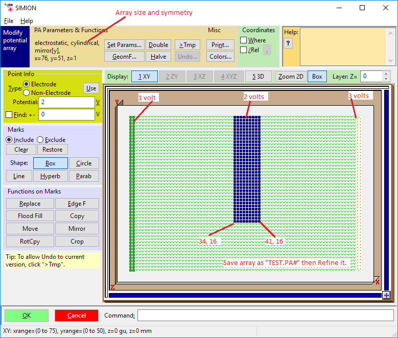
Click the New button and create a 76x by 51y by 1z 2D cylindrical electrostatic array.
Click the Modify button and use Modify to define the electrodes as show in the illustration below.

Note: If you have made an error in defining the array in New you can change the definition from within Modify (using the Set Params button).
When you’re satisfied that the results are OK, exit Modify by clicking the OK button.
The next task is to save the array as a fast adjust array (.PA#).
1. Click the Save button.
2. Make sure you are in the proper directory courses\short\session3\project (click the proper directory if needed) and Enter the name TEST.PA#
3. Optionally, a file memo (description) can be entered.
4. Click Save.
You will now be back on the Main Menu Screen. Click the Refine button to enter the Refine function.
Click the Refine button on the Refine Screen and SIMION will create and refine all the required fast adjust potential arrays.
Now click the Fast Adjust button (on the Main Menu Screen). SIMION will automatically load the TEST.PA0 file (your base solution file). Note: You could have loaded this file first via the Load button.
Set the left and center electrodes to 1,000 volts and the right electrode to 0 volts. Now click the Fast Adjust button to change the potentials in the TEST.PA0 array.
You will now be back on the Main Menu Screen. Click the View button to enter the View function. SIMION will automatically create a workbench volume the size of the potential array (TEST.PA0) assuming one mm per grid unit scaling.
Use various view orientations to look at the array including potential energy views.
Click the Define Particles button on the Particles tab to access ion definitions. Create a group of 11 positively charged ions (charge = +1) of color blue that start at x = 1 y = -5 (dy of + 1) with an energy of 0.01 eV. You can do this by setting “Source position = x,y,z”, setting “X = 1” and setting “Y” to an “arithmetic sequence” with “first = -5” and “step = 1”.
Click the OK button to return to View and fly the ions. They should focus. This is a converging acceleration lens.
Click the Define Particles button on the Particles tab to access ion definitions again.
Click the Add (group) button to create a copy of the current ion group.
Change the color of the second ion group to red, its charge to minus one, and the starting energy to 1050 eV.
Click the OK button and re-fly the ions. Use the PE view to see the negative ion surface. The positive ions see this lens as a converging acceleration lens, while the negative ions see this lens as a diverging deceleration lens.
Now open the PAs tab. Click the Fast Adjust button and change the center electrode potential to zero volts. Re-fly the ions view the results. You now have a diverging acceleration for positive ions and a converging acceleration for negative ions.

Electrostatic Lens Definition

Creating and Refining a Magnetic Potential Array

Remove All PAs From RAM
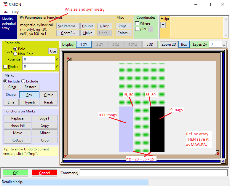
Click the New button and create a 51x by 100y by 1z 2D cylindrical magnetic array with ng = 20 (we plan to have a 20 grid unit pole gap).
Click the Modify button and use Modify to define the poles as show in the illustration below. Note: If you have made an error in defining the array in New you can change the definition from within Modify (using the Set Params button).
When you’re satisfied that the results are OK, exit Modify by clicking the OK button.
Now use Refine to refine the array (remember this is a normal PA not a fast adjust definition array).
Since this is not a Fast Adjust array we must save the refining results to keep them between sessions. Click the Save button and save the magnetic array as MAG.PA.
Enter View and look at the array.
One pole is 1,000 Mags, the other is 0 Mags, the pole separation is 20 gird units, and the value for ng is 20. Move the cursor to the center of the magnet and verify that the field intensity is 1,000 gauss. Note that the field intensity decreases quickly as you exit area between the poles.
Now try to define a group of 1,000 eV ions that pass between the poles and are bent by the magnetic field. This may take more effort than you expect because of the orientation of the potential array ( the x, y, and z workbench directions align with the array by default).
Once you get ions flying through the magnet use the Fast Adjust button on the PAs Option Screen to fast scale the field to some other field intensity and re-fly the ions.
You might also want to try expanding the workbench volume by clicking on the WrkBnch Tab and adjusting its size - be brave.

Demo of Using a Geometry File to Create an Array

Remove All PAs From RAM
Click the New button.
Click the Use Geometry File button and select the MAGNET.GEM file in the courses\short\session3 directory. SIMION will load and use the definitions in this .GEM file to create the same magnetic array you created in the example above.
Click the Modify button to verify that the array and its pole definitions were defined properly.
Let’s now take a quick look at a geometry file:
1. Click the GeomF button on the Modify Screen to access the Geometry file development system.
2. Click the Edit button to load the MAGNET.GEM file into a text editor (Windows Notepad by default).
3. Look at the file. These commands created and defined the potential array. More of this tomorrow.
4. Close the text editor.
5. Click the Cancel button to return to the Modify Screen.
Click the OK button to keep the array and exit Modify.
Refine the array (it is a simple .PA array).
Save the array as MAGNET.PA (needed to save solutions for use by .IOB file).
Remove All PAs from RAM.
Click the View button and load MAGNET.IOB and restore potentials.
Click the Define Particles button (within View screen Particlse tab) and load the MAGNET.FLY2 ion definition file.
Click OK to return to View and fly the ions.
This is an example of what is known as Z focusing. The entry points of the ions control whether they are focused or defocused in the z direction.

More for the Swift

Note that the orientation of the magnetic array is better in the demo than what you had. This is because the instance definition specified a different orientation. To examine it:

Click the PAs Tab in the Positioning panel note that the orientation of the array has been swung 90 degrees in the azimuth direction. Moreover the working origin of the potential array has been shifted a +25 grid units so that it is in the center between the two poles.
You should change this or that and see what happens. Leap!

Session 4 - Time-of-Flight Principles ¶

Basic Equations ¶

Simple Linear Time-of-Flight Equations

$KE = m v^2 /2$

$v_{mm/usec} = 13.891386 (KE_{eV} / m_{amu})^{1/2}$

$t = d / v$

$t_{usec} = d_{mm} ( m_{amu} /KE_{eV})^{1/2} / 13.891386$

Simple Reflectron TOF Equations

$t_{total} = t_{drift} + t_{reflectron}$

$t_{total} = d_{drift}/v + 2 v/a$

$a = f / m$

$f = work/distance = Volts/m$

$t_{total} = d_{drift} (m)^{1/2} /(2KE)^{1/2} + 2 (m)^{1/2} (2KE)^{1/2}/F$

$t_{total} = m^{1/2}(k1/KE^{1/2} + k2 KE^{1/2})$

Session 4 - Lab on Time-of-Flight ¶

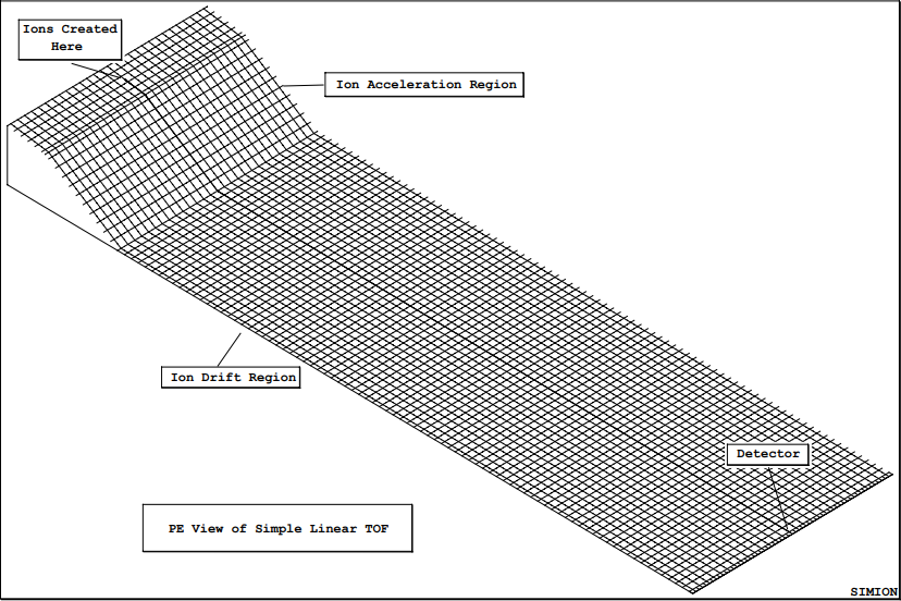
Flying Ions in a Simple Linear TOF

This Lab’s Files are found in Directory: courses\short\session4\linear

This model is used to demonstrate a very simple linear time-of-flight system. The demo makes use of voltage gradient time focusing for ions that are created at various locations in the ion formation region. The model is also used to demonstrate the use of the trajectory quality parameter to get proper discontinuity detection.

Creating the Required Files After Installation (First Time Only)

Remove All PAs From RAM
Use New and click the Use Geometry Files button. Use the LINEAR.GEM file by pointing to its button and clicking both mouse buttons ( in courses\short\session4\linear ).
Use the Save function to save the potential array as LINEAR.PA#.
Use the Refine function on LINEAR.PA# to create the required files for the demo.

Lab Steps Assuming the Required Files Have Been Created

Remove All PAs From RAM
Use View to load LINEAR.IOB from directory courses\short\session4\linear
Load the ions in the LINEAR.FLY2 file.
Set time markers on at 1.0 usec with their color set to 15 (so the ion’s markers use the same color as the ion’s trajectories).
Load the data recording file LINEAR.REC and turn data recording on.
Fly the ions singly with trajectory quality set to 2 (default value). Note the KE error. This value is too large. The ions must be missing a grid edge.
Re-fly the ions with increasing trajectory qualities (>2) until the KE error is around 10-6 or less. Notice that the error suddenly improves between two successive values of data quality. This is because the CV detection is now just sensitive enough to see the grid edge. Notice the improvement in the TOF times (on the data recording screen).
Notice that although the ions are created in different locations that they arrive at virtually the same time. However, the compensation is not perfect. Can you explain why? Are we dealing with problems with SIMION or basic physics?
Load and fly the ions in the LINEAR3.FLY2 file (25, 50, and 100 amu ions). Notice that all three ion masses bunch equally well.
Modify the data recording parameters so that the ion’s velocity is recorded when it splats. Are the velocity ratios correct between ions of different masses? Are the ion’s velocities correct (use the equations above and check array potentials.

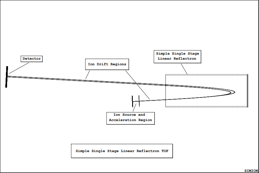
Using the Single Stage Linear Reflectron Demo

This Lab’s Files are found in Directory: courses\short\session4\reflect

This model is used to demonstrate a simple single stage linear reflectron time-of-flight system. The demo makes use of a single stage linear reflectron to time focus ions of the same mass but different kinetic energies.

No After Installation Files Need to be Created

Remove All PAs From RAM
Use View to load TOF.IOB from directory courses\short\session4\reflect
Load the ions in the TOF.FLY2 file.
Load the data recording file TOF.REC and turn data recording on.
Fly the ions grouped as dots. Note the arrival times on the data recording screen.
Click the PAs tab, set the instance to one (the reflectron mirror), and then click the Fast Adjust button. Record the current reflectron potential (should be 1000 V). Now increase the reflectron potential to 1500 volts and re-fly the ions. What happened? Now try 900 volts. Which ions get there first (low or higher energy)? Now try 1000.7 volts.
Select the detector instance (instance 3) on the PAs option screen. Click the Align checkbox (on Display tab) to align the workbench coordinates with the detector. Now fly the ions. Zoom in and watch them hit the detector. The dot speed slider can be used. Also try the single step function (“Step” button on the Particles tab).
Now go in and split the ion energies (was 50 eV between two ions in each group) to 25 eV delta for 3 ions in each group (increase the ions to 3 and change delta energy to 25 eV) for each of the two groups. Re-fly the ions. What does your time focusing look like now? Explain what you see - physics or SIMION?
Reload the TOF.FLY2 ion definitions file, delete the second ion group, and now load the TIMES.REC data recording file. Fly the two ions and use the data recording information to determine the ratio of drift time to time spent in the reflectron. The ratio should be 1.0 but it isn’t! What do you think is the cause? Hint: The acceleration stage creates a time shift.
To eliminate the impact of the ion acceleration stage, set its fast adjust voltage to zero (instance 2 - 800 volts by default), and then set the first ion’s KE to 801 eV. Now re-fly the ions. Now they are no longer time focused!
We can pull the source further back from the reflectron to help the time focus. Make sure the Align in unchecked. Select instance 2 (the source instance). Now check Align to align the workbench coordinates with the working origin of the source array instance.
On the PAs tab Positioning panel, move the source back by entering a negative value for Xwb (Hint: -91 is pretty close). The advantage of using the align function is that it allows us to move the source along the ion’s flight path. Thus no beam alignment problems.
Now re-fly the ions and check splat time-of-flights. They should be pretty close if you used -91.
Compare the drift time verses reflectron time ratios. They are very close to 1.0. If you fly an intermediate energy ion (e.g. 3 ions with 25 eV delta KE), its time ratios will be very close to 1.0.

How Refraction Impacts Time-of-Flight

This Lab’s Files are found in Directory: courses\session4\focus

This lab illustrates the errors in TOF introduced by the use of refractive elements like an einzel lens. A flat plane of ions entering an einzel lens does not leave as a flat plane of ions. However, the lab also demonstrates a trick that is useful to know.

No After Installation Files Need to be Created

Remove All PAs From RAM
Use View to load EINZEL.IOB from directory courses\short\session4\focus
Load and fly the ions in the EINZEL.FLY. Set time markers on a 1.0 usec, with marker color set to 15 (uses the ion’s color for marker color). Fly the ions singly as dots (fast - slider to right).
Note that while the ions enter the lens as a vertical line of dots they do not leave the einzel that way. Which ions are leading and which ions are trailing? What type of einzel is this: accel or decel? (Use PE view as an aid.)
Now fast adjust the center electrode to -250 volts and re-fly the ions. This is an accel einzel. Note that the ion distortion is reversed. Can you explain why the ion trajectories are time distorted the way they are?

This leads to an idea! Why not use two einzels in series to focus the ions while compensating for the time distortion by making one einzel an accel and the other a decel. If you want to test your skill with instances, go to the main menu, load the EINZEL.PA0 file and save it as EINZEL.PB0 (a second separate einzel fast adjust file). Remove All PAs from RAM and reload the EINZEL.IOB. Stretch the workspace to the right (increase xmax). Now mark where you want the second einzel to be, click the PAs tab, now the Add button and select the EINZEL.PB0 potential array. Use instance editing to scale and position this instance properly. Now make instance 2 an accel einzel and fly ions. If you play around with voltages the time focusing problem can be pretty much eliminated.

If you’re not that ambitious run the two einzel demo:

Remove All PAs From RAM
Use View to load FOCUS.IOB from directory courses\short\session4\focus
Load and fly the ions in the EINZEL.FLY2. Set time markers on a 1.0 usec, with marker color set to 15 (uses the ion’s color for marker color). Fly the ions singly as dots (fast - slider to right).
Zoom into the group of dots near the focus point. Notice the that the time distortion is minimal.
Use various views to examine how the distortions are removed as the ions fly.

Session 5 - Ion Cyclotron Resonance Mass Spectrometry ¶

Basic Equations ¶

The Cyclotron Frequency Equation

$\textrm{cyclotron frequency (Hz)} = f = q B / (2 \pi m)$

where:

$\textrm{q = charge * 1.60217733 E-19 C}$

$\textrm{B = magnetic field in Tesla } (\textrm{T} = 10^4 \textrm{ Gauss})$

$\textrm{m = mass = amu * 1.6605402 E-27 kg}$

Note that the cyclotron frequency of an ion is inversely proportional to it’s mass.

Session 5 - Lab on Ion Cyclotron Frequency Mass Spectrometer ¶

This lab’s files are found in directory courses\short\session5\icr .

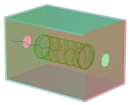
This lab is designed to demonstrate the trajectories of ions through an ion cyclotron resonance mass spectrometer. The model utilizes a three dimensional rectilinear ICR cell and a uniform magnetic field. User programs allow adjustment of the ion parameters and operating mode of the ICR. The workbench contains two overlapping instances: the electrostatic ICR cell (instance) and the magnetic field (instance). Initial ion conditions can be randomized by particle definitions. A user program allows the tuning parameters to be adjusted by the user during ion flying. The randomly assigned starting energies, positions, and directions are bounded by conditions set by the user.

Creating the Required Files After Installation (First Time Only)

Remove All PAs From RAM
Use New and click the Use Geometry Files button. Use the ICR.GEM file by pointing to its button and clicking both mouse buttons ( in courses\short\session5\icr).
Use the Save function to save the potential array as ICR.PA#.
Use the Refine function on ICR.PA# to create the required files for the demo.

Lab Steps Assuming the Required Files Have Been Created

Single Ion Trajectory

Remove All PAs from RAM. Use View to load the file ICR.IOB from the directory courses\short\session5\icr .
Load the trajectory file ICR_1.FLY2. This will fly a single ion of mass 1000. The ion will have a randomly selected starting position and angle, set via the particle definition.
Select trajectory quality = 0, ion as lines. Be sure rerun is not activated.
Default values of adjustable variables on the Variables tab will be used, except delay_start, which should be set to 20 (push the Fly’m button on this window). Fly the ion. The ion will start out and then an Rf field will be applied to the ICR cell to pump up the kinetic energy of the ion and get it moving at it’s cyclotron frequency. The ion will change from blue to red when the Rf is initiated, and from red to green when it is turned off. Stop the trajectory calculation after a brief period and view the trajectory from different orientations (they will stop automatically after max_time_usec microseconds). You can restart the ion several times at different orientations and get a good feel for what is happening to it. The ion moves back and forth between the trapping plates (end plates) while spiraling around the axis of the magnetic field.

Pumping Kinetic Energy into the ions - the Rf phase

Select the XY orientation and perform a 3D-Zoom of the area (-14,9) to (80,-9). Now switch to the XZ orientation and select the PE View. Start the ion flying and watch the potential energy surface as it varies with the Rf voltage. This is how the ion acquires the kinetic energy. When the pumping period ends, the potential is defined by the trap plate potentials, which keep the ion from wandering out of the cell.

Getting the Ions in Phase - groups of ions and separation by mass

In order to detect the ions they must be moving in phase inside the ICR cell. The RF pumping gives them the kinetic energy, and their mass determines their cyclotron frequency. This example demonstrates that ions of different mass are separated based on their cyclotron frequency.

Load the trajectory file ICR_3.FLY2; set the parameters to grouped, dots, slider to the right, rerun on, quality 0. Start a Fly’m; In the Variables tab push the Reset Values button to reset all of the variables. Fly the ions.
Select the XY orientation and watch as the ions are started, when they turn to red switch to the ZY orientation and watch as the two different groups are separated out. Note that one group is rotating at a higher frequency than the other. Which group should have the higher cyclotron frequency?

Measuring the Cyclotron Frequency with SIMION

In this example the theoretical cyclotron frequency will be compared against the SIMION calculated frequency. A single ion’s cyclotron frequency will be measured using markers and data recording.

Load the trajectory file ICR_W.FLY2. Open Data Recording (on the Particles tab).
1. At the top of the data recording window push the button marked Blank.
2. Push the check box labeled “Time of flight (TOF) (usec)” in the left section, and the check box marked “Crossing Plane Y=?” in the middle section. The time of flight (TOF) will be recorded each time the ion passes through the Y=0 plane.
3. Make sure Record data on the top is checked and click OK to exist this screen.

Set the trajectory parameters to lines (uncheck Dots), Rerun off, trajectory quality (T.Qual) 0, ZY orientation. Open the Log tab and click “W” to detach it in a new window. On the Variables tab, set the variables as defined below (be sure to note changes in the start and end mass):

variable

value

bx_gauss

30000

start_rht_voltage

0

capture_voltage

0

rf_voltage

20

starting_mass_amu

1950

ending_mass_amu

2050

rf_sweeptime_usec

120

start_delay_usec

1

pe_update_each_usec

1

Also observe in the Define Particles screen that X, Y, Z, KE, and direction are not randomized (unlike other .FLY2 files in this example).

Fly the ion. After it has made 5-6 full revolutions in the green phase, you can stop the ion (it is quite fast and will stop automatically after 1000 microseconds). Zoom in on the markers (red dots). Are the markers all perfectly aligned on the Y=0 axis? Why not? The variation in the time step at quality level 0 results in the marker (and data recording) occurring not exactly at Y=0, but within the time step that includes Y=0. Thus the variation is dependent upon the length of the time steps as the ions approach the Y=0 boundary.
Calculate the period for one revolution (using the numbers on the recording window). The theoretical cyclotron frequency for a 2000 amu ion in a 30,000 gauss field is 23.03417 kHz. How does this compare with the frequency measured using time markers? Calculate the ratio of Theoretical/SIMION.
Set the quality to 2 and rerun the trajectory. Zoom in on the time markers, do they all align now? Why? With the quality level at 2 the program performs a binary boundary approach to the Y=0 boundary. Recalculate the period and cyclotron frequency using the times in the data recording window. How does this compare to the Theoretical value?
Rerun the ion, in the Variables tab change the bx_gauss to 60,000 (double its original value). Now what is the cyclotron frequency? and how did this affect the radius? How would you use Data Recording to get a measurement of the radius?

Trapping ions formed outside the ICR cell

This example illustrates a method for trapping ions created outside the cell. Problems in trapping ions of widely varying mass due to their velocity differences are illustrated.

Load the ICR_4.FLY2 trajectories. Set to dots, grouped, slider to the right, quality 0, rerun on, XY orientation, and fly the ions. On the Variables tab, click Reset Values. Fly the ions. They will change color when the pump field comes on and when it is turned off. This works nicely for trapping these ions. What will happen when we have ions of widely varying mass?
Load the ICR_5.FLY2 trajectories and fly them as grouped dots with quality of 0, rerun on. The ions have been started with the same approximate kinetic energy (as set by the user defined variable). Note that the heavier ions (red) are not moving as fast as the lighter ions (blue) and that some of the blue ions enter and leave the cell before the trapping voltage is applied. How would you solve this problem?

Session 6 - Quadrupole Principles ¶

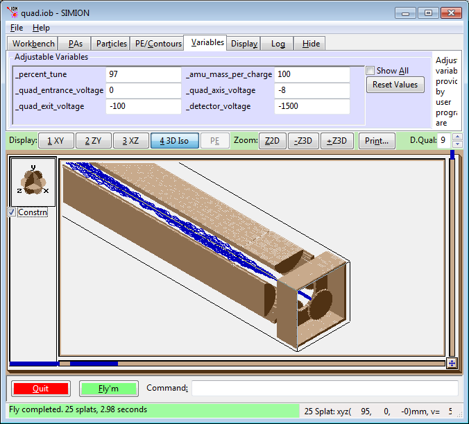
_images/quad_1.png — Fig. 86 quadrupole mass spectrometer¶

Basic Equations ¶

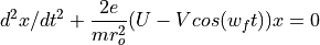
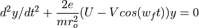
The Quadrupole Field Equations

$d^{2}x/dt^{2} + \frac{2e}{mr_o^2} (U - V cos (w_f t))x = 0$

$d^{2}y/dt^{2} + \frac{2e}{mr_o^2} (U - V cos (w_f t))y = 0$

$d^{2}z/dt^{2} = 0$

$2r_0 = \textrm{distance between opposing rods}$

$w_f = \textrm{angular frequency of applied field}$

$r_{circular\ rods} = 1.1487 r_o$

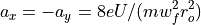
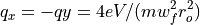
Determination of U and V via a_n and q_n

$a_x = -a_y = 8 e U / (m w_f^2 r_o^2)$

$q_x = -q y = 4 e V / (m w_f^2 r_o^2)$

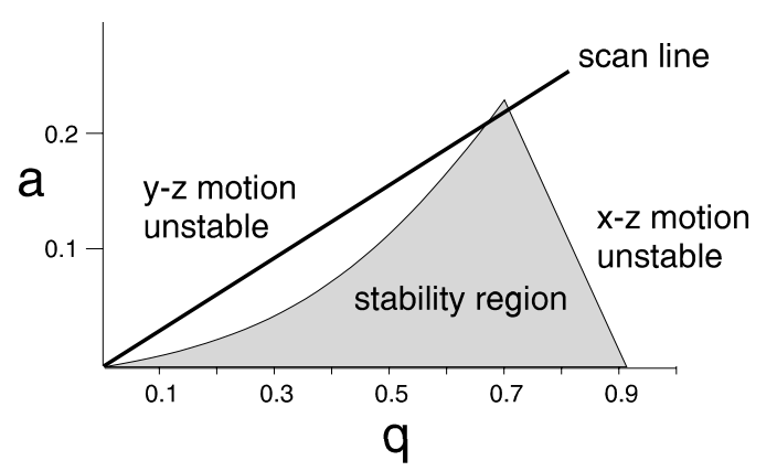
Quadrupole Stability Diagram ¶

Session 6 - Lab on Quadrupoles ¶

This Lab’s Files are found in Directory: courses\short\session6\quad

This lab is designed to demonstrate the trajectories of ions through a quadrupole mass spectrometer, and to illustrate the effects of tuning parameters on the trajectories and the transmission of the ions through the quadrupole. The model utilizes User Programs and the workbench feature of SIMION. It contains three different overlapping instances (pieces of the quadrupole) that are synchronized in their operation: The quadrupole lens (a 3D array), the quadrupole (a mirrored 2D array), and the exit lens with a plate detector (a 3D array). User programs randomize the ion initial conditions and allow the tuning parameters to be adjusted by the user during ion flying. The randomly assigned starting energies, positions, and directions are bounded by conditions set by the user.

Creating the Required Files After Installation (First Time Only)

Remove All PAs From RAM
Use New and click the Use Geometry Files button. Use the QUAD.GEM file ( in courses\short\session6\quad).
Use the Save function to save the potential array as QUAD.PA#.
Use the Refine function on QUAD.PA# to create the required files for the demo.
Remove All PAs From RAM
Use New and click the Use Geometry Files button. Use the QUADIN.GEM file ( in courses\short\session6\quad).
Use the Save function to save the potential array as QUADIN.PA#.
Use the Refine function on QUADIN.PA# to create the required files for the demo.
Remove All PAs From RAM
Use New and click the Use Geometry Files button. Use the QUADOUT.GEM ( in courses\short\session6\quad).
Use the Save function to save the potential array as QUADOUT.PA#.
Use the Refine function on QUADOUT.PA# to create the required files for the demo.

Lab Steps Assuming the Required Files Have Been Created

Remove All PAs from RAM. Use View to load the file QUAD.IOB from the directory courses\short\session6\group.
Examine the trajectory file QUAD.FLY2 (Particles tab > Define Particles). This will fly 25 ions of mass 100, the mass the quad is tuned to pass through. The ions will have randomly selected starting positions and angles as well.
Select trajectory quality = 0, ions as lines, ungrouped. Be sure rerun is not activated. No changes are made to the Variables tab.
Fly the ions (push the Fly’m button on this window).
View the ion trajectories using each view orientation, XY, ZY and XZ. In the XY view note the nodes that appear in the trajectories. In the XY view make a 3D zoom from X=5 to X=85 (leaving out the inlet and outlet optics), switch to ZY view and look at the trajectories.
In the ZY view make a cut that includes only the bottom and two side rods, switch to the 3D ISO view. Note the regions on the electrodes where the first instance interfaces with the second (the long quad rods), and where the second instance (the long quad rods) interfaces with the exit region.
Exit from View (use the Quit button on the left). In the main menu screen select the QUADIN.PA0 array and then select Modify. This takes you into the Modify screen where you can see how the geometry was defined. Select the XYZ view, note that is a planar array mirrored in X and Y. This saves array space (and memory!).
Leave Modify using the Quit button. Select the array QUAD.PA0 and look at it in Modify. What symmetries are used? Why? This is a simple 2D array–lots of space is saved by taking advantage of the symmetries of this system.
Leave Modify using the Quit button. Select the array QUADOUT.PA0 and look at it in Modify. What symmetries are used here?
Leave Modify using the Quit button.
Push the View button to return to the View screen. Push the PA tab and cycle through the instances (selecting each one in the list). Note they correspond to the three files you looked at in Modify. Instances can be added or deleted from the Workbench using the buttons on this window.

Mass Filtering - where do the ions go?

Load the trajectory file QUAD1.FLY2. This file contains three sets of ions, one of mass 95 (below the quad tune point, color red), one set at mass 100 (the quad tune point, blue), and a third set at mass 105 (green). Again the ions are started at random angles and starting positions. Fly the ions and observe the trajectories.
View the trajectories in the ZY view, note which set of quadrupole rods the lighter ions impact, and which rods the heavier ions impact. Look at this from different views. Do any of the lighter or heavier ions make it to the detector?
One of the user adjustable variables is the quadrupole axis voltage; this can be set on the Variables tab. Note the value (-8 volts) and run a set of trajectories. Write down the approximate positions in X where the light and heavy ions hit the rods. Now run the trajectories over and set the quadrupole axis voltage to -24 volts. How did this affect where the ions hit the rods, did any of the ions make it to the detector? What does this tell you about how the axis voltage may affect the peak resolution, the peak shape, and the signal intensity.
Load in the QUAD.FLY2 trajectory file and fly the ions with the quadrupole axis voltage set to -8 volts (default value), and in the XY view note the nodes that appear in the trajectories. Now re-fly the ions with this voltage set to -2 volts. How did this change the general shape of the trajectories, how many nodes appear now? Try other values of this voltage, what happens if this voltage is set positive? Could this be used to estimate the initial kinetic energy of the ions?

Ion Optics - how to get the ions into the quadrupole.

The effect of the ions’ trajectories as they enter the quad on the ion transmission is demonstrated. Dynamic display of potential fields is shown, and the manner in which SIMION handles trajectories at interfaces between different instances is demonstrated.

Load the QUAD.FLY2 trajectory file and fly the ions with the default adjustable Variables (hint, click Reset Values on the Variables tab before flying). Now re-fly the ions with the cone half angle increased to 15 degrees (this is on the Define Particles screen). What affect does this have? Notice that now many ions are lost. The acceptance ellipse for the quad is finite and small, ions that enter outside of this are lost.
Load the QUAD1.FLY2 file. Run the ions as dots with the speed slider all the way to the right, grouped, with rerun on, be sure trajectory quality is set to 0. View in the XY and YZ planes.
Switch to the XY view and make a cut from X=0, Y=0 to X=10, Y=-9. Switch to the XZ orientation and select PE View (potential energy surface). Set the drawing quality to 0 and the Gstep to 5 or higher. Fly the ions and watch the PE surface undulate. Switch back to the workbench view (PE button off), select ZY orientation, switch back to PE view, and watch again as ions fly.
Stop the Fly’m. Switch back to workbench view (PE button off), select XY orientation, zoom out one level and now make a second cut so you have the region (0,0) to (18,-9) zoomed into. Switch to XZ orientation and select the PE view and fly the ions. Notice that only the left side of the field is changing, the right side is staying constant. What happens when the ions finally get into the field on the right hand side? What happens when there are no longer any ions in the left hand region? Recall that the workbench has three instances in it, making up the quad. When does the program perform calculations for each PA instance? (Only when there are ions within an instance.) What happens when ions are in two PA instances?
Experiment with the effects of various tuning parameters (inlet and exit voltages etc), ion parameters (increase the energy spread, the position where ions are born) via the Variables.

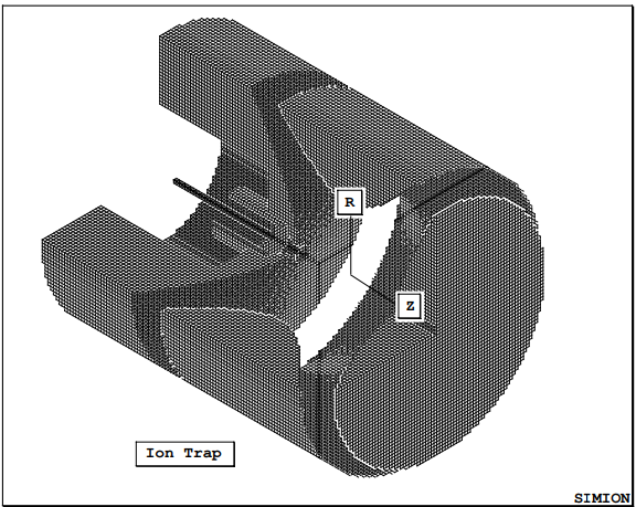
Session 7 - Ion Trap Principles ¶

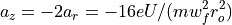
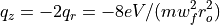
Basic Equations ¶

The Ion Trap Field Equations

$d^{2}z/dt^{2} - 4 z (U - V cos(w_f t)) e / (m r_o^2) = 0$

$d^{2}r/dt^{2} - 2 r (U - V cos(w_f t)) e / (m r_o^2) = 0$

$r_0 = \textrm{radius of trap}$

$w_f = \textrm{angular frequency of trap}$

Determination of U and V via an and qn

$a_z = -2 a_r = -16 e U / (m w_f^2 r_o^2)$

$q_z = -2 q_r= -8 e V / (m w_f^2 r_o^2)$

Ion Trap Stability Diagram

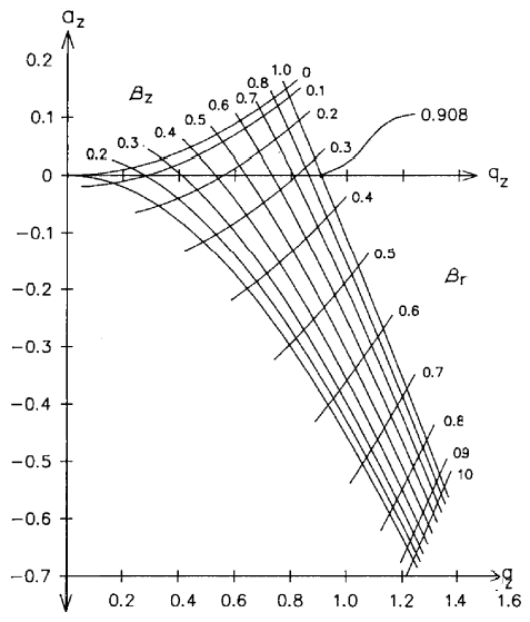
Secular Ion Motion Frequencies

$w_r = B_r w_f / 2$

$w_z = B_z w_f / 2$

$w_f = \textrm{trap frequency}$

Values for Bu in terms of a_u and q_u

$B_u = (a_u + z_u^2 / 2)^{1/2} \textrm{for} q_u < 0.4$

or in complete form

$B_u^2 = a_u + q_u^2/((2+B_u)^2 - a_u - q_u^2/((4+B_u)^2 - a_u - q_u^2/(...etc.))) + q_u^2/(( B_u - 2)^2 - a_u - q_u^2/((B_u - 4)^2 - a_u - q_u^2/(...etc.)))$

Session 7 - Lab on Ion Trap ¶

This Lab’s Files are found in Directory: courses\short\session7\group

Flying Ions in an Ion Trap

The first part demonstrates the trajectories of a single ion within a trap. The user programs allow the user to change the operating point of the trap (base mass, az, and qz) as the ion flies.

Creating the Required Files After Installation (First Time Only)

Remove All PAs From RAM
Use New and click the Use Geometry Files button. Use the TRAP2.GEM file by pointing to its button and clicking both mouse buttons ( in courses\short\session7\group).
Use the Save function to save the potential array as TRAP.PA#.
Use the Refine function on TRAP.PA# to create the required files for the demo.

Lab Steps Assuming the Required Files Have Been Created

Remove All PAs From RAM
Use View to load TRAP.IOB from directory courses\short\session7\group
Load and fly the single ion in the SINGLE.FLY2 ion group definition file (trajectory quality set to 0 for speed). Fly the ion as both a line and as a dot (use slider to vary dot speed). Notice that the ion has a different trajectory on every flight. This is because the user program randomizes the ion’s starting parameters automatically!
While an ion is flying, click the Variables tab to gain access to the user program’s adjustable variables. Change the _AMU_Mass_per_charge variable from its initial value of 40 to 90 then 100 and then 101 (the ion has a mass of 100). What happens?
Use the _Az_tune and _Qz_tune parameters to move the ion about in the stability diagram. Can you make the ion hit the ring electrode? How?
Use data recording to obtain the KE of the ion when it splats. Now fly 10-20 ions off the right edge of the stability diagram. Increase the mass of the ions to 500 and repeat. How does the ion’s mass impact its ejection energy?

The second part demonstrates interactions between ions flying in a trap. Factor charge repulsion as well as viscous cooling are used to demonstrate the formation of ion crystal patterns within the trap.

Load and fly the ten 100 amu ions in the GROUP.FLY2 file. Fly them as dots (fast - slider to right), grouped, with trajectory quality set to zero. Hit the Esc key to stop the flight. Re-fly the ions. Notice that they have different trajectories in every flight.
Now re-fly the ions with factor repulsion set to 1.0 (each ion just represents itself). The ion motions now include the effect of charge repulsion of the ions.
Now, while the ions are flying with charge repulsion active, Open the Variable tab to gain access to the user program’s adjustable variables while the ions are flying. Change the _linear_damping to 1.0. Notice that the trajectories collapse (ions are now being cooled). Zoom in. View the ion motions from the side and end-on. Notice that the 10 ions have formed a crystal pattern. Use dots and lines to see ion motions and streak patterns. Using a 3D volume zoom can be very helpful here. Change the factor repulsion to 1,000 so that each ion represents a cloud of 1,000 ions and see the change in the pattern size.
Load and fly the ions defined in GROUP1.FLY2 file with factor repulsion set to 1.0 and linear damping set to 1.0. There are 45 ions defined (15 -100 amu red, 15 - 200 amu green, and 15 - 300 amu blue). Notice the crystal pattern they form. Which ions are on the inside which ions are on the outside? Now change the _amu_mass_per_charge variable from 40 to 100 while the ions are flying. Notice the dramatic change in the edge view of the crystal pattern. Now bump the value to 102 and watch the 100 amu ions exit and the crystal reform. Interesting.

This Lab’s Files are found in Directory: courses\short\session7\tickle

Using the End Cap AC Voltages to Excite Selected Ions

If the end caps have a tickle voltage that has the secular frequency wz of specific ions’ mass for that a and q value the ions will gain energy and tend to leave the trap through the end cap holes. The user programs in this demo compute the proper tickle frequency and allow the user to change the tickle voltage and other parameters while the ions are flying. This demo also makes use of a collisional cooling model that uses mean free path and the mass of the cooling gas to simulate random collisional cooling of the ions.

Creating the Required Files After Installation (First Time Only)

Remove All PAs From RAM
Use New and click the Use Geometry Files button. Select the TRAP2.GEM ( in courses\short\session7\tickle).
Use the Save function to save the potential array as TRAP.PA#.
Use the Refine function on TRAP.PA# to create the required files for the demo.

Lab Steps Assuming the Required Files Have Been Created

Remove All PAs From RAM
Use View to load TRAP.IOB from directory courses\short\session7\tickle
Load and fly the ions in the TICKLE1.FLY2 (trajectory quality set to 0 for speed). Fly the ion as grouped as dots (fast - slider to right). One group of ions (black) are not affected (mass not in resonance). However, the other group of ions (blue - red) will eventually be blown out of the trap. Notice that these ions change from blue to red. The user program does this to indicate the polarity of the tickle voltage being placed on the end caps. This shows that forcing being applied to the ions.
Load and fly the ions in the TICKLE.FLY2 file (resonance ions only). Increase the tickle voltage and re-fly the ions.
Change the _amu_mass_per_charge variable from 40 to 80, re-fly and see what happens. Try flying ions with this variable set to 10 amu. Can you explain what you see?
Change the _amu_mass_per_charge variable from to 303, tickle to zero volts, and re-fly. Now turn on 2.0 volts of tickle while the ions are flying. This is an example of using tickle on the right stability edge to help eject ions.
This model makes use of a collisional cooling model based on mean free path assumptions controlling random collisions with a bath gas of a given mass (helium - 4 by default). Change the mean free path to 1 mm and see what effect increased gas pressure has on the tickle. Note setting mean free path to zero will turn off collisional damping.
You can also use the TRAP1.GEM file to create a new TRAP.PA# file with hole in left end cap and a grid over the hole in the right end cap. Save the array, refine it, Remove All PAs, reload the TRAP.IOB with View, and examine the impact of hole symmetry in the end caps on the preferred end cap for ion exit of the trap.

This Lab’s Files are found in Directory: courses\short\session7\inject

Injecting Ions into an Ion Trap

This demo models the injection of ions into an ion trap. 100 ions are injected singly and the user programs perform a Monte Carlo analysis of each ion’s fate. The model makes use of collisional cooling with mean free path and the mass of the cooling gas. It also includes an estimate of the reduction of the mean free path as a function of the ion’s mass (and assumed complexity):

$mfp_{est} = mfp/(1 + (n-1) \cdot \mathrm{\_Avg\_Visibility})$

Where:

$n = \mathrm{ion\ mass} / \mathrm{\_Avg\_Mass\_per\_atom}$

$\mathrm{\_Avg\_Mass\_per\_atom} = 12 \mathrm{(default)}$

$\mathrm{\_Avg\_Visibility} = 0.666 \mathrm{(default)}$

Creating the Required Files After Installation (First Time Only)

Remove All PAs From RAM
Use New and click the Use Geometry Files button. Select the TRAP1.GEM file (in courses\short\session7\inject).
Use the Save function to save the potential array as TRAP.PA#.
Use the Refine function on TRAP.PA# to create the required files for the demo.

Lab Steps Assuming the Required Files Have Been Created

Remove All PAs From RAM
Use View to load TRAP.IOB from the directory courses\short\session7\inject
Load and fly the ions in the INJECT.FLY2 (trajectory quality set to 0 for speed). Fly the ion as singly as dots (fast - slider to right). Fly about 30 ions and hit Esc to quit. Note the number of ions actually trapped (from the data screen).
The mean free path is set to 40 mm (approx 10-4 torr). Decrease the mean free path to 4 mm and re-fly the ions. Are the results what you expected?
Now change the mass of the ions from 100 (their default) to 500, mean free path to 40, and rerun 30 or so ions. How many did you trap? Not too many! Now re-fly these ions with the _amu_mass_per_charge variable set to 60 amu. Compare the results. Can you explain what you see?
You can also change the sample and focus ring potentials and see their impact on ion capture. Give the ions a lot of energy (sample potential) and see what happens.
You can also use the TRAP2.GEM file to create a new TRAP.PA# file with ideal grids across the end cap holes. Save the array, refine it, Remove All PAs, reload the TRAP.IOB with View, and examine the impact of grids. The options are endless.

This Lab’s Files are found in Directory: courses\short\session7\msms

Simulation of MSMS Fragmentation an Ion Trap

This demo models the use of tickle on the end caps to fragment a parent ion into a daughter ion. 100 Ions are injected singly and the user programs perform a Monte Carlo analysis of each ion’s fate. The model makes use of collisional effects of helium to fragment the parent ion. The model assumes this is a heating process that accumulates energy (most individual collisions are less than 0.1 eV). A fraction (user definable - assumed 0.5) of the collisional KE is assumed to be retained as heating of the parent ion. When this accumulated heating energy exceeds a designated value (10. eV by default) the ion is fragmented into its daughter ion. If the daughter ion is retained for 20 rf cycles (default) it is assumed to have been trapped.

Creating the Required Files After Installation (First Time Only)

Remove All PAs From RAM
Use New and click the Use Geometry Files button. Select the TRAP2.GEM file (in courses\short\session7\msms).
Use the Save function to save the potential array as TRAP.PA#.
Use the Refine function on TRAP.PA# to create the required files for the demo.

Lab Steps Assuming the Required Files Have Been Created

Remove All PAs From RAM
Use View to load TRAP.IOB from directory courses\short\session7\msms
Load and fly the ions in the MSMS.FLY2 (trajectory quality set to 0 for speed). Fly the ion singly as dots (fast - slider to right). Fly about 30 ions and hit Esc to quit. Note the number of daughter ions actually trapped (from the data screen).
The mean free path is set to 40 mm (approx 10-4 torr). Decrease the mean free path to 4 mm and re-fly the ions. Are the results what you expected?
Change the _amu_mass_per_charge variable from 40 to 10, mean free path = 40 mm, re-fly and see what happens. Try flying ions with this variable set to 60 amu. Can you explain what you see?
You can also use the TRAP.GEM file to create a new TRAP.PA# file with open end cap holes (both end caps). Save the array, refine it, Remove All PAs, reload the TRAP.IOB with View, and examine the impact of holes in the end caps on ion stability.

Session 8 - Creating 3D Arrays with Modify ¶

Discuss Modify with 3D Arrays (manual chapter 5 “Modify”)

2D to 3D and 3D to 2D Conversions
3D Layers and Marking in Modify
Find Options
Replace, Edge, Move, Copy, and etc.
Discuss the Double and Halve Functions

Class Lab:

Use Double and Halve and Inspect the Jags

Session 9 - Geometry Files ¶

What is a Geometry File

A geometry file is an ASCII file with the .GEM filename extension that contains the electrode/pole definitions for a potential array.
It also may contain the definition of the potential array: pa_define(100,20)

SIMION Functions that Use Geometry Files

The New function via the Use Geometry File button (makes use of pa_define commands).
The Modify function via the GeomF button (ignores pa_define commands for an existing array).

How Geometry Files Work

The geometry files contain a collection of fill commands.
Fill commands can define complex areas/volumes through the use of inclusion/exclusion commands (e.g. within and notin), orientation commands (e.g. locate), and large collection of basic shape commands (e.g. circle).
Each successive fill command has increasing priority. Later fill commands override earlier fill commands.
SIMION makes use of a geometry compiler to create an ordered fill search tree.
Each point within the array is checked to see if it is affected by a fill command (from last fill toward first fill).

The Geometry File Language

The Language is nested - commands fit inside each other.

e(1){fill{within{circle(0,0,5)}notin{box(0,0,2,2)}}}
e(1) ; electrode of one volt
{
fill ; fill command
{
within{ circle(0,0,5)} ; within a circle at 0,0 r = 5
notin{ box(0,0,2,2)} ; notin a box with corners of
} ; x,y: 0,0 and 2,2
}

Each command has its scope: The region of commands that are under its influence.
Commands can have parameters and/or scope
Inline comments begin with a semicolon.

The Logic Used in Fills

A point will be within a fills volume if it is contained in at least one of the fill’s within volume and not contained in any of the fill’s notin volumes.

e(1) ; electrode of one volt
{
fill ; fill command
{
within{ circle(0,0,5)} ; within a circle at 0,0 r = 5
within{ circle(20,0,5)} ; within a circle at 20,0 r = 5
notin{ box(0,0,2,2)} ; notin a box with corners of
; x,y: 0,0 and 2,2
notin{ box(20,0,22,2)}; notin a box with corners of
} ; x,y: 20,0 and 22,2
}

A point satisfies a within or notin if it is contained in the intersection volume defined by the shape commands within its scope.

within{circle(0,0,5) circle(5,0,5)} ; within intersection area notin{box(0,0,5,5) circle(0,0,5)} ; notin first quadrant

2D and 3D Considerations

All 2D shape commands (e.g. box and circle) are defined in x and y and have a +- 106 extent in the z direction when applied to 3D arrays.
All 3D shape commands (e.g. sphere) have their 2D intersection area (z = 0) when applied to 2D arrays.

Location, Scaling, and Orientation

Locate commands are used to locate, scale, and orient anything at any level. They even can be nested within themselves:

locate(100)
{
fill
{
within{sphere(0,0,0,50,60,40)}
notin{sphere(0,0,0,45,55,45)}
locate(0,0,0,1,0,0,-90)
{
notin{circle(0,0,10,5)}
}
}
}

Example above creates ellipsoidal shell with an elliptical hole vertically up through the center.

The pa_define Command

This command defines the potential array to use.
If it appears in a .GEM file it must be the first command.

It is used by the New command and ignored by the Modify Command

pa_define( nx, ny, nz, ; if nz = 1 then 2D array
  Symmetry, ; Planar or Cylindrical
  Mirroring, ; legal combinations of x,y,z, or none
  Type, ; Electrostatic or Magnetic
  ng) ; Value of ng parameter

The Geometry File Development System

Accessed from within Modify with the GeomF button.
Geometry files can be edited, test compiled and debugged.
Potential array can be erased (electrode/pole points removed).
Geometry definitions can be inserted into potential array.
Allows full manual control over translation, scaling and orientation via locate parameter panels (serves as outermost Locate command).

Session 9 - Lab on Geometry Files ¶

This Lab’s Files are found in Directory: courses\short\session9\trap

Inserting a Geometry File into Different Sized Arrays

The contents of a geometry file can be scaled to fit within arrays of different sizes. This lab shows how this is done

No After Installation Files Need to be Created

Remove All PAs From RAM
Use New to load TRAP.GEM from directory courses\short\session9\trap
Examine the array with View and then Modify.
The Array is 399x by 173y. Use Modify to halve the size of the array (200x by 87y);
Click the GeomF button to access the geometry file development system.
Test compile the geometry file by clicking the Compile button.
Change the Scale panel from 1.0 (default) to 0.5 to re-scale the geometry definitions to the smaller potential array.
Click the Erase Entire PA button then click the Insert into PA button. You should now be looking at the halved scale potential array.
Follow the above steps 4-8 with the appropriate numbers to halve the array again. What can you say about the change in resolution. Which array would you expect to model an ion trap more accurately?
Now we are going to insert this geometry file into a bigger array. In Modify, try to set a new array size of 797x by 345y. Did you have problems? What do you think is wrong? How would you fix it?
Remove All PAs From RAM
Use New to define a cylindrical electrostatic 2D array with 797x by 345y coordinates (you will have to increase the size of the Max PA to get these values).
Now enter Modify and Click the GeomF button.
Change the Scaling to 2.0 to double the geometry size to fit the new array.
Click the Erase Entire PA button then click the Insert into PA button. You should now be looking at the double scale potential array.
Click the Keep button and enter View. There are a lot of points in this array. Change drawing quality to 9 (click Esc if drawing takes too long).

This Lab’s Files are found in Directory: courses\short\session9\trap

Modifying the Trap Geometry File into a Stretched Trap

The contents of the trap geometry file above will be modified to define a Finnigan stretched trap which will be saved as the STRETCH.GEM geometry file

No After Installation Files Need to be Created

Remove All PAs From RAM
Use New to load TRAP.GEM from directory courses\short\session9\trap
Examine the array with Modify.
Click the GeomF button to access the geometry file development system.
Click the Edit button to edit the geometry file with EDY.
Rename the File STRETCH.GEM EDY keystrokes: Esc N STRETCH.GEM and press Enter
Now Let’s save the file, exit EDY and Select and use this file as the geometry file: Esc Q Y and your back in SIMION.
Click the Select button and click both mouse buttons on STRETCH.GEM to make it the currently selected .GEM file.
Use the Erase all points button and then the Insert into PA button to verify that the geometry file still makes the array OK.
Now the task is to shift both end caps 0.76 mm away from the trap center to create a stretched trap. The nominal scaling of this potential array is 0.1 mm/grid unit. Thus we need to shift the left end cap (and its contents) 7.6 grid units to the left and the right end cap 7.6 grid units to its right. The best strategy is to insert locate commands that have the proper shifts and enclose the proper electrode definitions. This will result in the caps being shifted properly. Go for it!
Assuming you’ve given it a good college try and failed. Use the Select button and click both mouse buttons on the STRETCH1.GEM file. Insert the geometry from this file. It works! Look at the file with EDY to see how it was done.

This Lab’s Files are found in Directory: courses\short\session9\einzel

Creating a geometry file for an EINZEL lens

A geometry file for an einzel lens will be created.

No After Installation Files Need to be Created

Remove All PAs From RAM
Load the EINZEL.PA# array with Load
Look at the electrode definitions with Modify.
Write down, on paper, the image of a geometry file that would create the einzel array. Try to include the proper pa_define if you can. Seek the assistance of an instructor as necessary.
Use New with the Use Geometry files button to access the file manager. Click the edit button to access EDY.
Name the file EINZEL.GEM with EDY: Esc N EINZEL.GEM then ENTER
Enter the contents into the file from the keyboard.
Now Let’s save the file, exit EDY, and Select and use this file as the geometry file: Esc Q Y and you’re back in SIMION.
Click both buttons on the EINZEL.GEM file’s button.
If all is OK the array will be created. If not, you will be informed.
In any event, enter modify and see what you created.
Click the GeomF button to begin to change or fix your geometry definitions
If you want to see a successful example, look at the EINZEL1.GEM file.

Session 10 - User Programs ¶

What is a User Program File

A user program file is an ASCII file with the .PRG filename extension that contains the user program segments for use with a potential array (.PA or .PA0).
It shares the name of the potential array it supports. TEST.PRG would automatically be used to support the TEST.PA array.
User programs are associated with arrays not instances.

How SIMION Utilizes User Programs

Each time the Fly’m button is clicked SIMION automatically compiles all user program files for any instances that have user programs attached to their associated potential array.
If Adjustable variables are found, the user will be given a screen to view and change their initial values.
User program segments are called only when ions are flying within the array that the user program segments support.

User Program Segments

The user program file contains user program segments.
User program segments act like subroutines.
SIMION calls each type of program segment at specific points in a trajectory calculation.
Thus you must use a specific user program segment to control a specific aspect of the trajectory calculation.

The Executable Program Segments

initialize
tstep_adjust
fast_adjust
init_p_values
efield_adjust
mfield_adjust
accel_adjust
terminate
other_actions
initialize_run (SIMION 8.1)
terminate_run (SIMION 8.1)
flym (SIMION 8.1)
load (SIMION 8.1)
instance_adjust (SIMION 8.1)

Where Program Segments are Used

flowchart.

[FIX:image]

Language Rules

Case is Ignored (upper and lower case are the same)
Blank lines and indentions are ignored
The Semicolon ; Starts an In-Line Comment
The language is based on the HP RPN calculator format with a 10 register rotary stack: 25 10 * 5 / ; means (25 * 10) / 5
The Compiler looks for words and converts them into Commands Numbers Variable Names and Labels

Examples of Commands

ke = speed_to_ke(speed, mass)

Converts from speed (mm/usec) to kinetic energy (eV). The first parameter is the ion’s speed and the second parameter is the mass of the ion (amu). Returns ion’s KE. This transform uses relativistic corrections. The ke_to_speed command performs the reverse transformation.

Classes of Commands

Calculations + - * / SIN COS LOG
Transformations deg rad rect3d_to_polar3d
Flow Controls if, while, for
Tests X==Y X~=Y X<Y X<=0 X>Y X>=Y
Communication to User and Variables print

Types of Variables

Adjustable Variables (defined at top of program file) adjustable MY_VARIABLE = 30.0 Global and lasts throughout a Fly’m
Local Variables (limited to scope or block they are defined in) local TIME_FLAG = -2.0E4
Reserved Variables ion_color ion_charge ion_px_mm Reserved variables are use to communicate with SIMION. Each program segment has specific read and write access to various reserved variables.

.	Name	Use	Units	Read Access	Write Access
.	adj_elect01 to adj_elect30	Fast Adj Electrode Voltages	Volts	fast_adjust	fast_adjust
.	adj_pole01 to adj_pole30	Fast Adj Pole Mag Potentials	Mags	fast_adjust	fast_adjust
.	ion_ax_mm ion_ay_mm ion_az_mm	Ion’s current Acceleration (WB Coordinates)	mm/ microsec2 (WB Orientation)	accel_adjust other_actions terminate	accel_adjust
.	ion_bfieldx_gu ion_bfieldy_gu ion_bfieldz_gu	Magnetic Field at Ion’s Location (PA’s Orientation)	Gauss (PA’s Orientation)	mfield_adjust	mfield_adjust
.	ion_bfieldx_mm ion_bfieldy_mm ion_bfieldz_mm	Magnetic Field at Ion’s Location (WB Orientation)	Gauss (WB Orientation)	accel_adjust other_actions terminate	None
.	ion_charge	Ion’s current charge	in units of elementary charge	Any Prog Seg	initialize other_actions
.	ion_color	Color of Ion	0-15	initialize other_actions	initialize other_actions
.	ion_dvoltsx_gu ion_dvoltsy_gu ion_dvoltsz_gu	Voltage Gradient at Ion’s Location (PA’s Orientation)	Volts/grid unit (PA’s Orientation)	efield_adjust	efield_adjust
.	ion_dvoltsx_mm ion_dvoltsy_mm ion_dvoltsz_mm	Voltage Gradient at Ion’s Location (WB Orientation)	Volts/mm (WB Orientation)	mfield_adjust accel_adjust other_actions terminate	None
.	ion_instance	Current Instance	1 - max instance	Any Prog Seg	None
.	ion_mass	Ion’s current mass	amu	Any Prog Seg	initialize other_actions
.	ion_mm_per_ grid_unit	Min Current Scaling1	mm/grid unit	Any Prog Seg	None
.	ion_number	Ion’s Number	1 - max ion	Any Prog Seg	None
.	ion_px_abs_gu ion_py_abs_gu ion_pz_abs_gu	Ion’s current PA Array Coordinates	grid units (PA’s Abs Coordinates)	Any Prog Seg	None
.	ion_px_gu ion_py_gu ion_pz_gu	Ion’s current (PA’s Coordinates)	grid units (PA’s Coordinates)	Any Prog Seg	None
.	ion_px_mm ion_py_mm ion_pz_mm	Ion’s current Workbench Coordinates	mm (WB Coordinates)	Any Prog Seg	initialize other_actions
.	ion_splat	Ion Status Flag2	Flying = 0 Not Flying != 0	initialize other_actions	initialize other_actions
.	ion_time_ of_birth	Ion’s Birth Time	microseconds	Any Prog Seg	initialize other_actions
.	ion_time_of_ flight	Ion’s current TOF3	microseconds	Any Prog Seg	other_actions
.	ion_time_Step	Ion’s Time Step4	microseconds	All but initialize	tstep_adjust
.	ion_volts	Electrostatic Pot at Ion’s Location	Volts	efield_adjust mfield_adjust accel_adjust other_actions terminate	efield_adjust
.	ion_vx_mm ion_vy_mm ion_vz_mm	Ion’s current Velocity (WB Coordinates)	mm/microsec (WB Orientation)	Any Prog Seg	initialize other_actions
.	sim_rerun_flym	Rerun Flym Flag	NO = 0 YES = 1	initialize terminate	initialize terminate
.	sim_update_pe_ surface	New PE Surface5	YES != 0	None	other_actions

UPDATE: SIMION 8.x expands this list. See Workbench Program Extensions in SIMION 8.1.

Session 10 - Lab on User Programs ¶

This Lab’s Files are found in Directory: courses\short\session10

Using an Existing User Program

The best way to start programming is to steal, steal, steal.

Remove All PAs From RAM
Use New to create a new array using EINZEL.GEM from directory courses\short\session10
Save the array as EINZEL.PA# and then Refine it.
Remove All PAs From RAM
Use View to load EINZEL.IOB
Use the Define button and load the EINZEL.FLY file.
Fly the ions and see that they focus properly.
In Windows Explorer, copy random.lua to einzel.lua.
Click Fly’m. SIMION will compile the user programs and display the adjustable variables. This uses default settings. What a mess!
You can turn off the user programs for a single run. Uncheck “Use program” on the Particles tab to turn the user program off, fly the ions, and enable it again.
Re-Fly the ions with various adjustable variable settings and see what happens. Are the results reasonable?

Adding a User Program Segment

User programs generally develop by evolution. In this can we would like to exert some user control from the keyboard. The object is to create a marker every time a keyboard key is pressed. This is really a very simple task.

Click User Program… on the Particles tab to edit the user program (einzel.lua).
Add the following two lines at the bottom of the file:
```
function segment.other_actions()
  if key() ~= 0 then
    mark()
  end
end
```
The first line defines the start of an other_actions program segment. The second line has some commands:

key() Tests for keyboard input and returns a non-zero key code if you hit a key

~= 0 Tests the return value from key() for a non-zero value (you hit a key) If the value is non-zero the next instruction will be executed (do if true) else it will be skipped and the program segment will exit without doing anything.

mark() This command creates a single marker. It uses the currently selected marker color and can be used as a trigger event for data recording. The mark command is executed if the ~= 0 test is true.

Fly the ions as dots with the speed slider to the center to slow the ions down a bit. Hit the spacebar and watch for markers. Can you create markers anywhere? What is the problem? Remember, an array’s user program will only be called when ions are actually within its instance’s array volume.

Additional Challenges

Modify the user program to output the ion’s x, y, and z position in workbench coordinates (mm) when you hit a key. Hint: The print command is helpful.
Change this program to output x, y, and z in 3D array coordinates and then in absolute array coordinates.
For a real challenge calculate and display the ion’s KE when you hit a key. Hint: The polar3d_to_rect3d and speed_to_ke transforms might be helpful.


[Optional] Your name:	email:	phone: