Poisson Equation¶

Definition¶

The Poisson equation when applied to electrostatic problems is

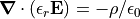
$\bnabla \cdot (\epsilon_r \vec{E}) = -\rho / \epsilon_0$

for electric field $\vec{E}$ , relative permittivity $\epsilon_r$ (dielectric constant), Space Charge density $\rho$ , and electric constant $\epsilon_0$ .

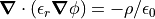
It can also be written in terms of potential, $\phi$ :

$\bnabla \cdot (\epsilon_r \bnabla \phi) = -\rho / \epsilon_0$

Without dielectrics, it becomes

$\bnabla^2 \phi = -\rho / \epsilon_0$

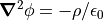
Without space-charge either, it becomes the Laplace Equation.

The Poisson equation can be thought of as the differential form of Gauss’s Law:

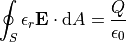
$\oint_S \epsilon_r \vec{E} \cdot \textrm{d}A = \frac{Q}{\epsilon_0}$

as the boundary surface (S) volume approaches zero, thereby converting the surface integral into a divergence operator. The space-charge is the source of the field divergence.

The Poisson equation can also be used for various other problems, including magnetic and current density ones, the heat equation, etc. See “Applications” in Poisson Solver in SIMION.

SIMION Specific Notes¶

The Refine function in SIMION 8.1 (unlike previous versions) supports solving the Poisson equation. 8.1.1.0 added dielectrics support.

For further details on the new Poisson solving capabilities, see the Poisson Solver in SIMION. Some screenshots of examples are shown below.

Please note, however, that being able to solve the Poisson equation is a necessary but often insufficient condition for solving Space Charge problems involving particle trajectories that cause the space-charge. Situations like this typically involve iterative approaches, such as

Solving trajectories without space-charge, solving the Poisson equation given the space-charge in the previously calculated particle trajectories, re-solving the trajectories with the previously calculated space-charge distribution, etc., repeating this until a convergence is reached.
Solving one or a couple time-steps without space-charge, solving the the Poisson equation given the space-charge in the previously calculated particle trajectories, solving one or a couple more time-steps with the previously calculated space-charge distribution, etc., repeating until the trajectories are done.

Some user program examples are included that provide a basis for automating such things, but at this time it is currently somewhat involved and considered advanced and experimental (i.e. assembly and technical know-how required). (However, this was much improved in 8.1.0.45.)

Examples¶

Computation of field with known space-charge density distribution¶

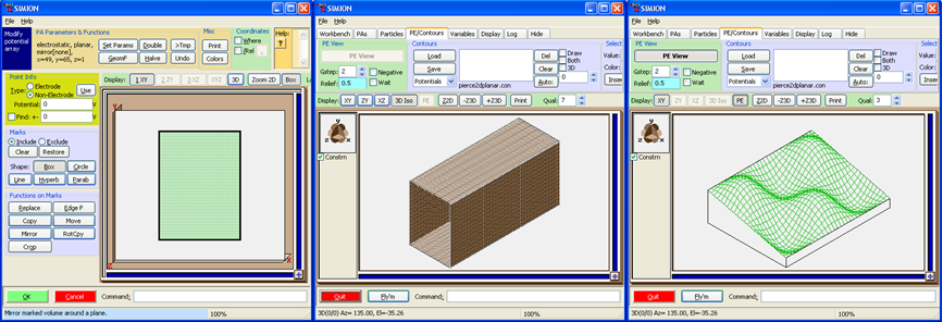
The following shows a conductive rectangular tube (2D planar) with a known (sinusoidal) space-charge density inside. This tube is modeled with a potential array, as usual, and the charge density is modeled with a charge density array that defines charge density (C gu^-2 mm^-1) in each grid cell. A user program created these arrays and refined the potential array while passing the charge density array as an option. As shown, the space-charge density causes local minima and maxima in the potential plot where there is high negative and positive charge density respectively.

Computation of field and trajectories together¶

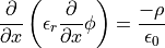
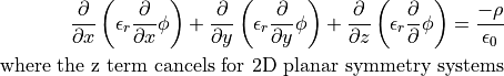
The following is a simulation of a Pierce gun (2D planar or cylindrical). A beam of electrons travels from the cathode to anode. In the absence of space-charge (low current beam) the potential contour lines are curved inward, and the beam diameter narrows. In the presence of space charge (high current beam), the space-charge of the particles trajectories alter the potential contours so that they become straight and the beam travels horizontally. In the below simulation, whenever the beam advances approximately 1 grid unit, a workbench user program updates the charge density array, rerefines the potential array given the charge density array, and also updates the display of the contour lines. The simulation with space-charge density disabled (in which the beam narrows) is also shown for comparison.

Reference Notes¶

The Poisson equation in 1D coordinates is

$\frac{\partial}{\partial x} \left( \epsilon_r \frac{\partial}{\partial x} \phi \right) = \frac{-\rho}{\epsilon_0}$

The Poisson equation in 3D Cartesian coordinates:

$\frac{\partial}{\partial x} \left( \epsilon_r \frac{\partial}{\partial x} \phi \right) + \frac{\partial}{\partial y} \left( \epsilon_r \frac{\partial}{\partial y} \phi \right) + \frac{\partial}{\partial z} \left( \epsilon_r \frac{\partial}{\partial } \phi \right) = \frac{-\rho}{\epsilon_0} \textrm{where the z term cancels for 2D planar symmetry systems}$

The Poisson equation in 2D cylindrical coordinates:

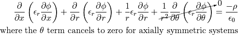
$\frac{\partial}{\partial x} \left( \epsilon_r \frac{\partial \phi}{\partial x} \right) + \frac{\partial}{\partial r} \left( \epsilon_r \frac{\partial \phi}{\partial r} \right) + \frac{1}{r} \epsilon_r \frac{\partial \phi}{\partial r} + \cancelto{0}{ \frac{1}{r^2} \frac{\partial}{\partial \theta} \left( \epsilon_r \frac{\partial \phi}{\partial \theta} \right) } = \frac{-\rho}{\epsilon_0} \textrm{where the } \theta \textrm{ term cancels to zero for axially symmetric systems}$

These are all found by substituting the cooresponding forms of the grad and div operators into the vector form of the Laplace operator, $\bnabla \cdot \left( \bnabla \phi \right)$ , used in the Poisson (or Laplace) equation. See also Wikipedia:Del_in_cylindrical_and_spherical_coordinates.


[Optional] Your name:	email:	phone: