Monte Carlo Method

Monte Carlo methods are a way to do numerical calculations by means of statistical random sampling. The stereotypical example is calculating the constant by means of recording the proportion of darts hitting inside a circle circumscribed in a square dart board, assuming darts hit the board with uniform randomness. Monte Carlo methods tend to be simple to use but relatively slow to achieve accuracy. For general background, see Wikipedia:Monte_Carlo_method.

SIMION-Specific

Monte Carlo methods can be of importance theoretically in certain aspects of SIMION operation.

A particle beam may contain an enormous number of particles in practice (1 amp being 6.241 x 10¹⁸ elementary charges per second). Rather than simulating every particle from this population, you will normally only simulate a small representative sample of particles from a much larger population (to use statistical terminology). There are many valid ways to select this sample. The particles may be uniformly randomly chosen from within the volume of the particle beam (Figure 1B) or they may be regularly spaced within that volume (Figure 1A). (Note: The sampling in 1A is deterministic, not random, and therefore not exactly Monte Carlo.) Moreover, it’s not even necessary that the sampling be uniform over the volume: in a beam with cylindrical symmetry you may sample particles evenly along the radius (r) in a cross-sectional plane containing the axis (1D), in which case you should weight the particles by a factor of r in any type of calculation on them (e.g. current density plots) if you want them to be statistically representative of the particles in the beam. An alternative to Figure 1D is 1E, where instead of weighting particles we concentrate their density as a function of r (i.e. is made to be uniformly distributed rather than r). Moreover, the density of particles in your physical beam may not be uniform but rather Gaussian distributed, and there are two ways to handle that: the position of the particles may be selected from a Gaussian distribution (Figure 1C) or you may select particles from a uniform distribution (Figure 1A, 1B, or 1D) but assign each particle an appropriate weight. SIMION Example: secondary has some similar notes concerning modeling of changes to beam current across secondary emission.

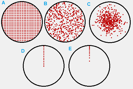
Fig. 80 Figure 1: various ways to sample particles from the cross-section of a particle beam.

In FLY2 File particle definitions, which were used to generate the above figures, there are various options to define sequences and distributions. See the FLY2 Appendix of the SIMION 8.0/8.1 manual for details. This includes arithmetic sequences in X, Y, and Z positions (like 1A and 1D); uniform (random) distributions in X, Y, and Z; circle distributions (like 1B); and Gaussian distributions (like 1C). You can also define your own distributions, either calculating them from an external program for import from an ION File or using FLY2 capabilities for custom distributions (Issue-I407). The “weighting” of particles (mentioned above) can be done via the “charge weighting factor” (CWF, see SIMION manual index) in the particle definitions. CWF affects things like repulsion (SIMION Example: repulsion and SIMION Example: poisson make use of it) but can also be outputted in Data Recording for your own use (e.g. you might use this when making current density plots).

Not only are particle positions statistically distributed but often also energies, velocity distributions, masses, charges, and time-of-birth (TOB).

In many cases, only the envelope rather than interior volume of the beam matters, in which case it’s not important that the particles be statistically representative. However, in cases of Space Charge, such as in using the Poisson Solver in SIMION (or the older charge repulsion methods), it is particularly important that particles simulated are statistically representative of your physical distribution of particles because the particles are used to represent charge density distribution in space, which is fed back into the Poisson solver (or charge repulsion methods).

Another area where Monte Carlo methods come up are in Ion-Gas Collisions (non-vacuum conditions).

SIMION also has Monte Carlo numerical integration library (simionx.Integration - Numerical integration routines), which the SIMION Example: gauss_law example uses to compute a Gauss’s Law surface integral. The Monte Carlo approach is mainly just a convenience here.

Accuracy of Monte Carlo methods depends on the size of the sample. One rough estimate of error due to use of Monte Carlo methods is to rerun the calculation more than once (using a different random sample each time) and compare the results. You can also compare the results as a function of the number of particles run and examine the convergence (like in SIMION Example: gauss_law).

Other Tips

Rotation

If the electrodes and beam both have 2D cylindrical symmetry, it may be more convenient for visualization/analysis to fly the particles within a 2D plane. If the particles in the beam are sampled in 3D (e.g. FLY2 circle distribution like in Figure 1A or 1B), you could use a workbench user program like below to rotate the particles around the x-axis back to the Z=0 plane (like in Figure 1E):

simion.workbench_program()
local function rotate()
  local theta = -math.atan2(ion_py_mm, ion_pz_mm)
  ion_py_mm, ion_pz_mm =
     math.cos(theta)*ion_pz_mm - math.sin(theta)*ion_py_mm,
     math.sin(theta)*ion_pz_mm + math.cos(theta)*ion_py_mm
  ion_vy_mm, ion_vz_mm =
     math.cos(theta)*ion_vz_mm - math.sin(theta)*ion_vy_mm,
     math.sin(theta)*ion_vz_mm + math.cos(theta)*ion_vy_mm
end
function segment.initialize()
  rotate()
end
function segment.other_actions()  -- optional
  rotate()
end

The other_actions segment rotates particles back to the Z=0 plane on every time step. This segment may be omitted if the z component of the particles’ velocity is always zero, in which case the particles always remain in the Z=0 plane after being placed in the Z=0 plane by the initialize segment.

An alternative to the initialize segment above is to rotate the particles in the FLY2 file, as shown in Rotating particles in cylindrical symmetry to 2D plane.