Paraxial Approximation
In analyzing lens systems, it can be helpful to make the approximation,
referred to as the paraxial appoximation [3],
that the distance r and angle  of rays from the optic axis is small. This can allow
approximations such as
of rays from the optic axis is small. This can allow
approximations such as  and
and  .
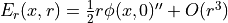
In a cylindrically symmetric lens, we may also assume
that the radial force is a linear function of r by ignoring
.
In a cylindrically symmetric lens, we may also assume
that the radial force is a linear function of r by ignoring  terms in the series expansion
 [1].
Transfer Matrix methods can also be applied. The term occurs in other areas as well, notably light optics
[4] [5].
[1].
Transfer Matrix methods can also be applied. The term occurs in other areas as well, notably light optics
[4] [5].
SIMION-specific: SIMION does not impose the paraxial approximation because it can just as well, in the general case, perform a complete calculation of the ray (direct ray tracing), but the paraxial approximation is still a useful concept for describing and reasoning about systems, and it can be observed. See also Lens and SIMION Example: lens_properties.
As an example, load the SIMION Example: einzel (3D cylindrical Einzel lens) and execute these lines in the command bar (using the SIMION 8.1 simion.pas API):
pa = simion.wb.instances[1].pa
vpp = (pa:field_vc(44,0,0) - pa:field_vc(42,0,0))/2
for y=0,18 do local ex,ey,ez = pa:field_vc(43,y,0); print(y,ex,ey,-vpp*y/2) end
The output is
0  0.00044623609977634  -0                -0
1  0.00044428927495233  -0.17781293264966 -0.17765444177787
2  0.00043840684034535  -0.35588612396623 -0.35530888355574
3  0.00042866422852228  -0.53440720053051 -0.53296332533361
4  0.00041519012360425  -0.71337103479918 -0.71061776711149
5  0.00039816206681564  -0.89249053069886 -0.88827220888936
6  0.0003778052310679   -1.0710844420651  -1.0659266506672
7  0.00035438893978323  -1.2479573211516  -1.2435810924451
8  0.00032822043240799  -1.4212758476776  -1.421235534223
9  0.00029963579692094  -1.5884533017798  -1.5988899760008
10 0.00026899862027108  -1.7460625920167  -1.7765444177787
11 0.0002366972330492   -1.8898080997316  -1.9541988595566
12 0.00020313782007975  -2.0145954910926  -2.1318533013345
13 0.00016874647809573  -2.1147421766658  -2.3095077431123
14 0.00013397228273959  -2.1843626535966  -2.4871621848902
15 9.926759618395e-005  -2.217935562564   -2.6648166266681
16 6.5083447026382e-005 -2.2110096583242  -2.8424710684459
17 3.1859044696603e-005 -2.1609408204639  -3.0201255102238
18 -0                   -0                -3.1977799520017
Notice that at low values of radius (y, also known as r), the second column is fairly constant and the last two columns (for measured and estimated radial field component) match closely.
Related topics: Picht equation [2] [1] and paraxial ray equation.