Using Poisson Superfish with SIMION¶

Poisson Superfish a finite element (FEM) field solver and set of programs for static and RF electromagnetic fields in 2D planar or 2D cylindrical symmetry.

Shown here is how to import magnetic fields computed in Poisson or Pandira and exported by SF7 into SIMION.

Why Import?¶

Magnetic fields are important to SIMION because magnetic fields affect the particle trajectories (Lorentz Force Law) simulated by SIMION. Various types of instrumentation and mass spectrometers simulated by SIMION incorporate magnetic fields. So, we need to determine the magnetic field. Calculation of magnetic fields can be a little complicated, and SIMION has some magnetic capabilities (Magnets), but SIMION is more established in the area of particle optics and electric fields than magnetic problems, so there are times we may want to import magnetic fields from other packages, typically based on the finite element approach (FEM). You may prefer the FEM approach and the magnetic capabilities provided in Poisson Superfish, so we ask how to export those fields from Poisson Superfish and import them into SIMION for particle optics handling and other analysis.

In SIMION we are typically most interested in ultimately knowing the B field rather than the H field since the B field is used for calculating particle motion by the Lorentz Force Law. Nevertheless, it is also possible to import other quantities like the H field or $\mu$ if you so desire.

SIMION and Poisson Superfish Versions¶

It is recommend that you use SIMION version version 8.1.2.7 or above because that includes SIMION Example: poisson_superfish demonstrating the importation for fields from Poisson Superfish into SIMION. It also recommended using SIMION 8.2-2014-03-14 or above because it includes the latest version of a field library (Field Functions Library (simion.experimental.field_array)) that makes the importation and magnetic vector potential A handling a bit easier, and the examples and this discussion utilize it. Nevertheless, it is possible to do much of this in earlier versions using SIMION Example: field_array in SIMION 8.0/8.1 and the SIMION Example: contour (contourlib81) in SIMION 8.1, though you are more on your own.

These examples were tested in Poisson Superfish version 7.17 but probably will also work in older and newer versions as well. If not, let us know, and necessary minor adjustments could be made.

Methods of Import¶

The basic approach¶

There is more than one way you may import magnetic fields into SIMION. Although you could import the B field vectors directly, it is suggested to instead import the magnetic vector potential A. (There is not a simple provision for exporting the magnetic scalar potential from Poisson Superfish.)

We also will normally import the field data as points on a uniform rectilinear grid rather than finite element mesh format since the former is conveniently represented as a regular SIMION potential array (PA) object, making it convenient and efficient to view and manipulate in SIMION.

Import vector magnetic potential¶

One means of importing the magnetic field into SIMION is to import the vector magnetic potential A. B can then be expressed in terms of A by the equation $\v{B} = \curl \v{A}$ , which SIMION largely takes care of for you. For 2D problems, this A is convenient because only one dimension of the A vector is non-zero (the z, or “azimuthal”, component perpendicular to SIMION’s 2D xy plane), so it can be treated as a scalar A, whereas B is a vector. We can import A into a single SIMION potential array (PA), whereas to import B directly we would need two potential arrays, one for each scalar component of the 2D vector. For 2D cylindrical PA’s we will actually typically import r*A, where r is the radial distance from the axis (y coordinate in SIMION). (The use of the multiplying r factor under cylindrical symmetry is a typical convenience, as noted on Magnetic Potential.)

Now, SIMION magnetic potential arrays normally don’t store vector magnetic potential A or r*A but rather a form of scalar magnetic potential V defined as $\v{B} = - \grad V$ . Therefore, if we store A or r*A rather than V in the magnetic PA, we need to slightly re-express the B that SIMION computes. The necessary adjustment can be seen from the following equations. The required adjustment is automatically taken care of by a SIMION utility library we will use, so if you don’t follow that math don’t worry:

$\v{B} = - \pd{V}{x} \uv{x} - \pd{V}{y} \uv{y} = - \grad V \textrm{ (planar and cylidrical)} \v{B} = \pd{A}{y} \uv{x} - \pd{A}{x} \uv{y} = (\grad F) \times \uv{z} \textrm{ (planar)} \v{B} = \frac{1}{r} \pd{(r A)}{r} \uv{x} + \frac{-1}{r} \pd{(r A)}{x} \uv{r} = \frac{1}{r} (\grad F) \times \uv{z} \textrm{ (cylindrical)}$

Poisson Superfish SF7 can export A for 2D planar and 2D cylindrical and A for cylindrical (axisymmetric) symmetry, Poisson Superfish reports the values of r and A in units of cm and gauss respectively, whereas SIMION units are mm and gauss respectively, and the conversion routines converts between cm and mm automatically.

Import B Field Vector Components¶

Another approach would be to import $B_x$ and $B_y$ components of the magnetic field, each as a separate PA (e.g. “bx.pa” and “by.pa”). This is similar the SIMION Example: field_array (SIMION 8.1) and is also demonstrated in the SIMION Example: poisson_superfish (bmag.iob). This approach is less recommended because it requires two arrays and does not afford plotting the field lines as directly. This approach may be easier though if not using SIMION 8.2, which has the simple Field Functions Library (simion.experimental.field_array) utility library for computing B from A.

There are two ways to go about this. The simpler way is to export the data using the Poisson Superfish SF7 program (OUTSF7.txt) and then import that into SIMION as a PA or PA’s. The other way is to have SIMION read the data directly from the binary solution file (.t35). The former approach has the advantages of PAs, such as speed and visualization. The latter avoids interpolating onto a rectangular grid but rather reads and interpolates directly from the finite element mesh, so it has some improved accuracy and directness.

Exporting from Poisson Superfish¶

The following process can be used to export field data from Poisson Superfish into a text file that SIMION can then convert into a SIMION potential array (PA).

First go through the usual steps to solve the field. Create an Automesh file (.am) and run it in Automesh (e.g. by double clicking the file in Windows Explorer). This creates a binary solution file (.t35) as well as a an Automesh log file (OUTAUT.TXT). Solve the .t35 file in Poisson or Pandira (e.g. by right clicking the file in Windows Explorer and selecting Run Poisson or Run Pandira). You can view the resultant .t35 in WSFplot (e.g. by double clicking the .t35 file).

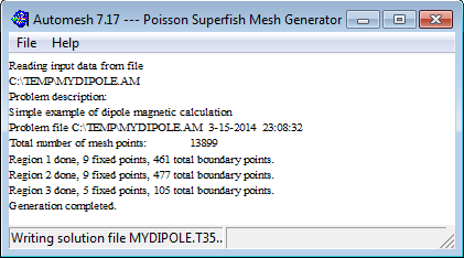
_images/psf_automesh.png — Fig. 31 Running Automesh on the Automesh file (.am) to generate the binary solution file (.t35).¶

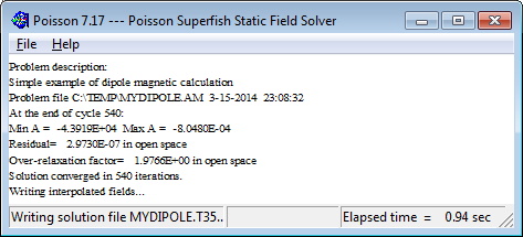
_images/psf_poisson.png — Fig. 32 Running Poisson to solve the binary solution file (.t35).¶

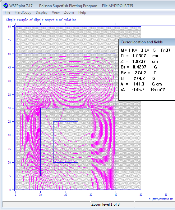
_images/psf_wsf.png — Fig. 33 Viewed the solved solution file (.t35) in WSFPplot.¶

We can export potentials or fields to a rectangular grid in a text file using the SF7 Interpolator program (e.g. by right clicking the .t35 file and selecting Interpolate (SF7).

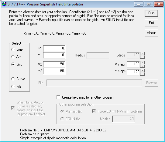
Select the “Grid” option to export a 2D rectangular grid of points, which is most suitable for converting to a SIMION PA. Specify the lower-left (X1, X2) and upper-right (Y1, Y2) points of the rectangle to export (the initial values are the full size of the problem space and may be suitable). Specify the number of steps in the X and Y directions. Note that this represnts the number of grid cells along each dimension. The number of points is one more than this. For example, if X1=0 and X2=50 and X steps=100, then there are 100 grid cells, each of size 0.5 cm, and 101 grid points surrounding those grid cells.

The grid cell size should probably be roughly the size of the triangles in your Poisson Superfish mesh, or perhaps a little smaller for increased accuracy. If the exported cell sizes are much larger then than the Poisson Superfish mesh triangles, you will likely introduce significant interpolation error (if it is ok to throw away accuracy, then why not calculate your Poisson Superfish mesh at lower resolution?). If the exported cell sizes are much smaller than the Poisson Superfish mesh triangles, then this increases memory usage and conversion time while likely not increasing accuracy significantly since the largest source of error in the field may be due to the size of mesh in Poisson Superfish itself rather than in the interpolation on the SIMION PA. If in doubt, you can experiment with different cell sizes and see how small the cells need to be to keep their effect on SIMION results within a desired threshold. You would set the X and Y steps such that the grid cells are roughly square (triangles in your Poisson Superfish mesh are probably not too oblong either), though SIMION 8.1 no longer requires grid cells to be perfectly square (Anisotropically Scaled Grid Cells in SIMION).

The SF7 will write a text file named “OUTSF7.TXT” containing your data. It will have various text including something like this

Magnetic fields for a rectangular area with corners at:
(Rmin,Zmin) = (0.0,0.0)
(Rmax,Zmax) = (50,60)
R and Z increments:   100   120

      R             Z              Br            Bz            |B|           A           dBz/dr        dBr/dz        Field
    (cm)          (cm)             (G)           (G)           (G)         (G-cm)        (G/cm)        (G/cm)        Index
   0.00000       0.00000      0.000000E+00 -2.734250E+02  2.734250E+02  0.000000E+00  0.000000E+00  0.000000E+00  0.000000E+00
  0.500000       0.00000      0.000000E+00 -2.733921E+02  2.733921E+02 -6.835209E+01  1.306702E-01  1.306702E-01 -2.389794E-04

Note that the file indicates the field type (magnetic or electric), the symmetry (2D cylindrical RZ or 2D planar XY), and bounds of the array (Rmin,Zmin) and (Rmax,Zmax) in cm, the number of grid cells (R and Z increments), and the field data at each grid point. The field data includes most importantly the non-zero scalar component of magnetic vector potential (A) in units of G-cm. It also includes the B field vector (Br,Bz), as well as derivatives of the field (which we normally ignore).

Converting to a SIMION PA¶

The library psflib.lua in SIMION Example: poisson_superfish (in SIMION 8.1.2.7 or above) can be used to convert a text file exported from Poisson Superfish into a SIMION potential array (PA). It can be as simple as executing this from the SIMION command bar:

PSF= simion.import 'c:/Program Files/SIMION-8.1/examples/poisson_superfish/psflib.lua'
PSF.convert('c:/temp/OUTSF7.txt', 'F.pa')

Alternately, you may want to add something like this to your workbench user program:

simion.workbench_program()
local PSF = simion.import 'c:/Program Files/SIMION-8.1/examples/poisson_superfish/psflib.lua'
function _G.regenerate()
  PSF.convert('c:/temp/OUTSF7.txt', 1)
end

Now, anytime you enter regenerate() from the SIMION command bar within the View screen, PA instance #1 will be automatically recreated from the file OUTSF7.txt. This can be convenient if you need to edit the field in Poisson Superfish and re-export it to SIMION multiple times. You may need to resize the SIMION workbench (e.g. Min button on Workbench tab) or refresh the screen after regenerating.

The convert function has the following interface:

function convert(infile, out, col, polecol)

Converts a Poission Superfish SF7 text file into a SIMION potential array (PA).

infile is that absolute or relative path to the OUTSF7.TXT text file to import.
out can be the absolute or relative path to the SIMION PA file to write. If out is a SIMION PA, PA instance object (e.g. simion.wb.instances[1]), or PA instance number (e.g. 1), then the field is imported into that existing object.
col is the column of from which values are imported. It can be a number (positive integer) column index or it can be a string that matches the description or notation string in a column header (e.g. “”). If omitted, it defaults to 6 (V, Az, or A). (Note that columns 1 and 2 are assumed to be coordinates.)
```
1     2     3      4        5         6
R(cm) Z(cm) Er(cm) Ez(V/cm) |E|(V/cm) V(V)
X(cm) Y(cm) Ex(cm) Ey(V/cm) |E|(V/cm) V(V)
X(cm) Y(cm) Bx(G)  By(G)    |B|(G)    Az(G-cm) dBy/dy(G/cm) dBy/dx(G/cm) dBx/dy(G/cm)
R(cm) Z(cm) Br(G)  Bz(G)    |B|(G)    A(G-cm)  dBz/dr(G/cm) dBr/dz(G/cm) Field (Index)
```
The column identifir ‘rA’ is also supported, which multiplies A by r.
mirror indicates any additional mirroring that should be added to the PA. This is a combination of ‘x’, ‘y’ (e.g. ‘xy’). 2D cylindrical arrays only support ‘x’ (since ‘y’ is implied). If omitted, it defaults to ‘’ (no additional mirroring).

If you are imporing Bx and By (or Bz and Br) field components directly, they you will need to convert the two arrays individually:

PSF = simion.import 'c:/Program Files/SIMION-8.1/examples/poisson_superfish/psflib.lua'
PSF.convert('c:/temp/OUTSF7.TXT', 'Bx.pa', 'Bz')  -- or 'Bx'
PSF.convert('c:/temp/OUTSF7.TXT', 'By.pa', 'Br')  -- or 'By'

or, again, if you prefer:

simion.workbench_program()
local PSF = simion.import 'c:/Program Files/SIMION-8.1/examples/poisson_superfish/psflib.lua'
function _G.regenerate()
  PSF.convert('c:/temp/OUTSF7.txt', 1, 'Bz')
  PSF.convert('c:/temp/OUTSF7.txt', 2, 'Br')
end

Note that for 2D cylindrical coordinates, the SIMION’s x and y coordinates are z and r respectively in the SF7 output (or y and x respectively in the original Automesh file)

Warning: You should not ever Refine the PA imported into SIMION. The field is already solved, and Refining it will clear the field because the boundary conditions are not properly defined in the PA. In fact, SIMION will give a warning if you attempt to do so:

WARNING: This PA is not intended to be refined.
Refining will likely clear/corrupt it.
Details: This PA had been marked as not refinable (i.e. pa.refinable = false).
Some possible reasons for this are that the array is already refined but the
boundary conditions were removed from the PA or the array is being used in an
unconventional way to hold data not understood by Refine."

If desired, you can enable X and/or Y mirror planes on the PA:

PSF.convert('c:/temp/OUTSF7.txt', 1, 'Bx', 'x')  -- X mirror
PSF.convert('c:/temp/OUTSF7.txt', 1, 'Bx', 'xy') -- Y and Y mirror

(This can alternately be done via the Set button on the Modify screen but is most convenient to do in the convert function as shown above.)

Viewing the PA in SIMION¶

Once you add the PA to the workbench (View screen), you can use the PE and Contour functions in the usual way to plot the fields:

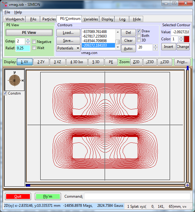
Note that the potential contours and the values with label Mags in the status bar are with units of gauss mm² ng (A*r, for 2D cylindrical PA’s) or gauss mm ng (A, for 2D planar PA’s). (The unitless magnetic scaling factor ng is normally 1, or at least the conversion library makes it so.)

Beware that any B values displayed in the status bar or Data Recording are actually $- \grad \v{F}$ , where F=A or F=r*A, which is probably not really what you want. Also any values of $|\v{B}|$ displayed are $|\grad \v{F}|$ , which are the same as $|\v{B}|$ for 2D planar symmetry but are $r |\v{B}|$ for 2D cylindrical symmetry. In the screenshot above, the $|\grad \v{F}|$ value is about 2824 gauss*mm but since this is 2D cylindrical symmetry it must be divided by the radial distance y=10.3 mm to obtain about 274 gauss as the value for $|\v{B}|$ .

Applying the B Field to Particles¶

The particles will not properly see and interpret the B field in the PA of magnetic vector potential. They are not aware that the values in the PA are not scalar magnetic potential but rather vector magnetic potential. In fact, if you used Data Recording to record the B field the particles see, you will observe it is not correct. We can rectify this with a short workbench user program that defines an mfield_adjust segment to override the B field with one properly interpreted from the PA (a future update to SIMION will eliminate the need for this user program, but for now this is the quick adjustment).

If you have a 2D planar PA storing the z component of magnetic vector potential $A_z$ , then just attach the following short user program to the SIMION workbench. (As usual, click User Program... from the Particles tab, paste the code into the file, and save.)

simion.workbench_program()
local A = simion.experimental.field_array{Az=1}
segment.mfield_adjust = A.mfield_adjust

If this is a 2D cylindrical PA storing r A, then replace the name Az with rA:

simion.workbench_program()
local A = simion.experimental.field_array{rA=1}
segment.mfield_adjust = A.mfield_adjust

If you have two PAs containing the Bx and By components of the B field, do something like this:

simion.workbench_program()
local B = simionx.experimental.field_array{1,2}
segment.mfield_adjust = B.mfield_adjust

Note: the above assumes PA instance numbers 1 and 2 (as displayed in the PA Instances list on the PAs tab) represent the Bx and By field components respectively; if not, change the numbers in the code accordingly. Likewise for the other examples above.

(Note: The Field Functions Library (simion.experimental.field_array) library requires SIMION 8.2-2014-03-14 or above.)

You can now define particles, Fly them, and Data Record in the usual way in SIMION. Below shows the vmag.iob example in SIMION Example: poission_superfish. For simplicity of demonstration, only a single particle is flown.

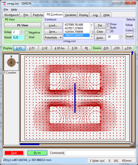
_images/psf_export_vtraj.png — Fig. 34 2D view of flux function (F=rA) contour lines (red) and particles (blue).¶

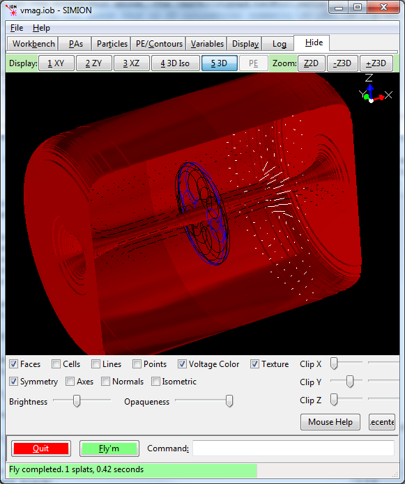
_images/psf_export_vtraj2.png — Fig. 35 3D view (SIMION 8.2) of magnetic vector potential contour surfaces (red) and particles (blue), as well as contour library field vector planes (white and black).¶

Plotting with the Contour Library¶

Besides PE/Contour functions, you can use the SIMION 8.1 contour library (SIMION Example: contour). This will plot vector fields and is especially useful if importing the B field vectors directly since there you don’t have a scalar potential to plot.

simion.workbench_program()
local B = simionx.experimental.field_array{1,2}
segment.mfield_adjust = B.mfield_adjust

local CON = simion.import 'c:/Program Files/SIMION-8.1/examples/contour/contourlib81.lua'
CON.plot{func=B.bfield, mark=true, npoints=20, z=0}
print('TEST', B.bfield(10,0,0))  -- read single point (mm, gauss)

The bfield property on the field array object is a function representing the B field, suitable for plotting or testing, and works with field arrays created from B and A. Some of the examples in SIMION Example: poisson_superfish utilize the contour library.

Checking the Conversion¶

It is strongly recommended to confirm that the field imported into SIMION is approximately the same as the field in Poisson Superfish in case some simple error was made in the conversions of physical dimension units, magnetic potential units, symmetry, or poor grid cell size. The rule in SIMION and any simulation program is “always be suspicious.”

First make a visual check. Draw contours in SIMION to see the field and ensure it looks qualitatively similar, as they are in the figures above and below. Also hover your mouse over the field in SIMION to measure physical dimensions to ensure they are the same as in Poisson Superfish WSFplot.

Note that SIMION dimensions are by default in units of mm, whereas in Poisson Superfish they are in cm.

Check the value of the B field on at least one point in both programs and compare. The WSFplot program can be used to read the field value at the given point by hovering the mouse over it. Alternately you can read field at exact points from the OUTSF7.TXT file.

In SIMION, you can add something like this to your workbench user program:

simion.workbench_program()
local A = simion.experimental.field_array{rA=1}
print('TEST', A.bfield(90, 30, 0))

or just copy and paste this one-liner on the command bar:

=simion.experimental.field_array{rA=1}.bfield(90, 30, 0)

(Be careful to specify “rA” or “Az”.)

The B field (x, y, and z components) will display in the status bar (or remove the “=” and wrap it inside a print( ) command like previously to write it to the Log window tab).

If flying particles, also check that the particles see that correct B field. Define an mfield_adjust segment as described previously, fly some particles and use the standard Data Recording features to measure the B field observed by the particles at some position (convenient places are Ion's Start, Ion's Splat and Crossing Plane. This confirms that everything is operational.

Some difference in the QuickField and SIMION field is expected due to the differences in interpolation. This error can be reduced by decreasing the Grid Cell Width and Height values in the QuickField export, as discussed previously.

Pole/Non-Pole PA Point Types and Particle Splatting¶

The default is to import the field without any information of pole/non-pole point types. So, you will not see the poles during visualization (apart from the contours), nor will particles see the poles for splatting purposes (unless of course you have an electrostatic PA or user program causing the splatting). The OUTSF7.txt file does not contain the pole information. You could redraw it in the Modify screen (e.g. Find/Replace and Change point type only). If you just way drawing, see the section below.

Drawing Regions¶

The region boundary stored in the automesh output file (OUTAUT.TXT) can be drawn in the SIMION graphical window to assist in visualization. This can be done by adding a line like this to the workbench user program:

simion.import 'psflib.lua'.draw{path='OUTAUT.TXT', painst=1}

The PA instance number (#1) should be a PA instance created from the convert function above. The region boundary lines will be positioned (translated/rotated/scaled) in the same way as this PA instance.

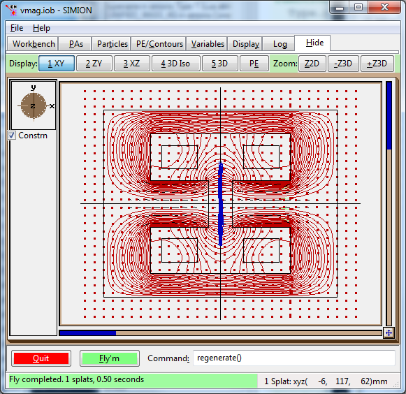
_images/psf_draw.png — Fig. 36 Example of drawing boundaries (black) from the OUTAUT.TXT file, in addition to the fields and trajectories.¶

The draw function has the following interface:

function draw {path=path, painst=painst, swap=swap, color=color, mark=mark}

Draw region boundaries to graphics window given in Automesh file (OUTAUT.TXT).

path - relative or absolute path to Automesh output file (OUTAUT.TXT).
painst - PA instance created from the SF7 output. This is used to properly position (translate/rotate/scale) the Automesh geometry onto the View screen. It can be a PA instance object (e.g. simion.wb.instances[1]) or PA instance number (e.g. 1). The geometry is positioned the same way the PA instance is positioned. If omitted (nil), no repositioning is done.
swap - whether the X and Y coordinates from the Automesh output file are to be swapped (true/false). This is typically used for 2D cylindrical coordinates, where Y is the axis of symmetry in Poisson Superfish and X is the axis of symmetry in SIMION. If omitted (nil), this will be automatically set to true if 2D cylindrical symmetry is used and false if 2D planar symmetry is used. The symmetry is referred from painst, or if that is omitted, from the Automesh output file.
color - color number (0..15) in which to draw region lines with. If omitted, it defaults to 0 (black).
mark - whether to draw markers on region boundary logical points (true/false). If omitted, it defaults to false.

Converting Magnetic Vector Potential to Magnetic Scalar Potential¶

You may for some reason want a PA with magnetic scalar potential rather than magnetic vector potential. There does not appear to be an option of exporting the magnetic scalar potential directly from Poisson Superfish. It is not even always possible to do this uniquely on the whole domain, like when you have current sources.

The SIMION function simion.experimental.spotential_from_vfield() (see spotential_from_bfield.iob in SIMION Example: magnetic_potential) may be used to convert a known B field to magnetic scalar potential (over at least some of the domain) by integration. This is not normally recommended and may introduce some loss in accuracy too but can be done.

Reading Fields Directly from the Binary Solution File (.T35)¶

Rather than using SF7 to export the .T35 data to an OUTSF7.TXT file and then importing that into a PA, we can instead read the .T35 data directly from a workbench user program and apply the field with an mfield_adjust (or efield_adjust) segment. This requires SIMION 8.2. An example is shown in the vmag.lua (SIMION Example: poisson_superfish) but initially is commented out:

local PSF = simion.import 'psflib.lua'
segment.mfield_adjust = PSF.mfield_adjust_from_t35('mydipole.t35', 'x', 1)
-- optional plot or test field too...
local field = PSF.field_from_t35('mydipole.t35', 'x', 1)
CON.plot {func=field, mark=true, npoints=30, z=0}
print('TEST', field(0,0,0))

Before using that, you will need to copy the Poisson Superfish fld_msvc.dll file into your c:\Program Files\SIMION-8.1\x32\lib\ folder and run the 32-bit SIMION c:\Program Files\SIMION-8.1\x32\simion.exe. This DLL is only supported on the 32-bit SIMION.

The library supports these functions:

field = PSF.field_from_t35(path, antimirror, painst)

Returns field (field) function electric or magnetic field in Poisson Superfish
binary solution file (.t35).
path - relative to absolute path to .t35 file.
antimirror - antimirror planes ('', 'x', 'y, or 'xy').  Default is ''
painst - PA instance (either object, e.g. simion.wb.instances[1], or instance
  number, e.g. 1).  If specified, field will be re-positioned
  in the same way as the PA instance.  If ``nil``, not re-positioning is done.


efield_adjust = PSF.efield_adjust_from_t35(path, antimirror, painst)

Returns efield_adjust segment from electric field in Poisson Superfish
binary solution file (.t35).
path - relative to absolute path to .t35 file.
antimirror - antimirror planes ('', 'x', 'y, or 'xy').  Default is ''
painst - PA instance (either object, e.g. simion.wb.instances[1], or instance
  number, e.g. 1).  If specified, field will be re-positioned
  in the same way as the PA instance.  If ``nil``, not re-positioning is done.


mfield_adjust = PSF.mfield_adjust_from_t35(path, antimirror, painst)

Returns mfield_adjust segment from magnetic field in Poisson Superfish
binary solution file (.t35).
This is similat to efield_adjust_from_t35 but for magnetic fields.


Az, Bx, By, DBYDY, DBYDX, DBXDY = PSF.interp(path, x,y)

Reads field data from Poisson Superfish binary solution file (.t35)
at point (x,y) cm.
path - full or relative path to .t35 file.
Bx,By - magnetic field in gauss or electric field in V/cc.
Az - magnetic vector potential in G-cm or electric voltage in V.
DBYDY, DBYDX, DBXDY - derivatives of Bx and By.

The meaning of the variables depends on the problem type (see SF7 program output):
For 2D planar magnetic: Az, Bx, By, |B|, dBy/dy, dBx/dy, and dBy/dx. (dBx/dx = dBy/dy)
For 2D cylindrical magnetic: A_phi Br Bz, |B|, dBz/dr, dBr/dz,
  and field index n = (r/Bz)(dBz/dr)
For 2D planar electrostatic: V, Ex, Ey, and |E|
For 2D cylindrical electrostatic: V, Er, Ez, and |E|
For 2D planar RF: Ex, Ey, |E|, and Hz
For 2D cylindrical RF: Ez, Er, |E|, and H_phi

Note: for 2D cylindrical problems, r is x and z is y.
A units are gauss-cm. B units are gauss.
V units are volts. E units are V/cm.

Returns nil if point outside of problem space.
Raises error on other problems.


val = PSF.variable(path, name)

Reads variable from Poisson Superfish binary solution file (.t35).
path - full or relative path to .t35 file.
name -- name of variable to retrieve.
val - real number, or nil if variable doesn't exist.


[Optional] Your name:	email:	phone: