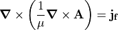
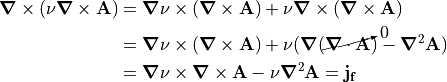
Magnetic Potential
Overview
Magnetic potential refers to either magnetic vector potential (A) or
magnetic scalar potential ( ).
Both types of magnetic potential are alternate ways to re-express the
magnetic field (B) in a form that may be more convenient for
calculation or analysis.
This is similar to how the electric field (E) can be
conveniently re-expressed in terms of electric potential (
).
Both types of magnetic potential are alternate ways to re-express the
magnetic field (B) in a form that may be more convenient for
calculation or analysis.
This is similar to how the electric field (E) can be
conveniently re-expressed in terms of electric potential ( ).
A is a type of vector potential
related to B via
).
A is a type of vector potential
related to B via  .
However, is a type of scalar potential
related to B via
.
However, is a type of scalar potential
related to B via  , but, unlike magnetic
vector potential, its use is limited to cases such as regions
of zero free current density.
In contrast, electric potential () is a type of
scalar potential
related to the electric field (E) via
, but, unlike magnetic
vector potential, its use is limited to cases such as regions
of zero free current density.
In contrast, electric potential () is a type of
scalar potential
related to the electric field (E) via  .
Magnetic potential is often more complicated than electric potential
due to its often vector nature and complicated effects of magnetic
materials (e.g. hysteresis).
.
Magnetic potential is often more complicated than electric potential
due to its often vector nature and complicated effects of magnetic
materials (e.g. hysteresis).
SIMION Simulation Capabilities
SIMION 7.0-8.1.0 have traditionally only handled magnetic scalar potential, with poles of infinite permeablities, which can be modeled with magnetic PA’s and solved with the Laplace Equation (Refine). SIMION 8.2 already has some capabilities to handle variable permeability in magnetic scalar potential, as well as magnetic vector potential with currents. These can be solved under the Poisson Equation with the Poisson Solver in SIMION and are demonstrated in SIMION Example: magnetic_potential. These capabilities are described below.
Magnetic Vector and Scalar Potential - Theory
The following is a summary of the theory of magnetic potential, including the equations and conditions under which it can be solved numerically, such as with SIMION. This is only an overview. Additional background is available in standard reference books like Griffiths, as well Wikipedia: Magnetic_potential.
According to the Maxwell Equations [1],
magnetic B fields
may or may not be rotational (i.e.  ), depending on conditions,
but they are always divergenceless (i.e.
), depending on conditions,
but they are always divergenceless (i.e.  ).
Since any divergenceless field can be re-expressed as the curl of some other vector field
(albeit not uniquely),
we therefore define a magnetic vector potential (A) according to
.
The rationalle for using A is that we have useful tools for computing
A, and upon finding A we can easily determine B from this definition.
).
Since any divergenceless field can be re-expressed as the curl of some other vector field
(albeit not uniquely),
we therefore define a magnetic vector potential (A) according to
.
The rationalle for using A is that we have useful tools for computing
A, and upon finding A we can easily determine B from this definition.
The magnetic B field is closely related to the magnetic H field
by  , where
  is the
magnetization.
is related to the bound current density
is the
magnetization.
is related to the bound current density  (e.g. in permanent magnetic material),
whereas
(e.g. in permanent magnetic material),
whereas  is related to the free current density
  ,
as seen by the Maxwell Equations under time independent conditions.
Problems can be more conveniently solved in terms of H since often
,
as seen by the Maxwell Equations under time independent conditions.
Problems can be more conveniently solved in terms of H since often
 not
not  is known.
Applying an H field to a material may induce a magnetization in that material,
and this relationship may alternately be written
is known.
Applying an H field to a material may induce a magnetization in that material,
and this relationship may alternately be written
 , where
 is the permeability.
Permeability is a scalar constant in the simplest case but in general it may be a function
of environmental factors including the field, it may be a tensor, and it
may have hysteresis (memory effects).
Permeability may alternately be expressed in terms
of its reciprocal, the reluctivity
is the permeability.
Permeability is a scalar constant in the simplest case but in general it may be a function
of environmental factors including the field, it may be a tensor, and it
may have hysteresis (memory effects).
Permeability may alternately be expressed in terms
of its reciprocal, the reluctivity  . We may also speak of relative
permeablity or relative reluctivity:
. We may also speak of relative
permeablity or relative reluctivity:  ,
,
 .
.
Combining the above  (time-independent),
, and gives
(time-independent),
, and gives
We seek to solve A given known distributions of
 and in space and
known boundary conditions on A. We can then determine B from A.
and in space and
known boundary conditions on A. We can then determine B from A.
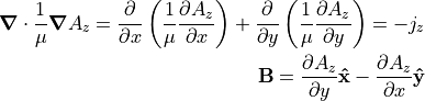
If is constant, then in 3D Cartesian coordinates,
the above equation can be rewritten [2] as
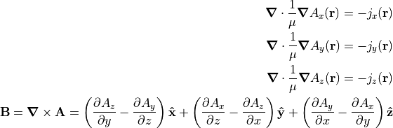
That is three separate instances of the Poisson Equation with scalar variables, each solvable independently with the Poisson Solver in SIMION (SIMION Refine, SIMION 8.2).
If is not constant, then
which is not presently solvable in SIMION in the general case but is in specific cases given below.
In 2D planar coordinates ( need not be constant),
where only the z components of A and are
non-zero, 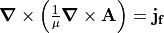 becomes a single Poisson equation:
In 2D cylindrical coordinates  , where only the azimuthal
() components of A and j are
non-zero, this also resembles a single 2D planar Poisson equation:
, where only the azimuthal
() components of A and j are
non-zero, this also resembles a single 2D planar Poisson equation:
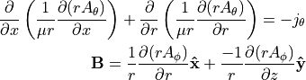
where we actually solve for  .
.
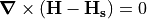
In regions where (free) current density is zero,
the H field is irrotational
(i.e.  ), and irrotational fields can also be
represented as a gradient of a scalar
potential, so in this case we can define the magnetic scalar potential
as
), and irrotational fields can also be
represented as a gradient of a scalar
potential, so in this case we can define the magnetic scalar potential
as  . Equivalently, .
Magnetic scalar potential is analogous to electric potential ().
Combining this expression for B with gives
. Equivalently, .
Magnetic scalar potential is analogous to electric potential ().
Combining this expression for B with gives
 ,
which is the Poisson Equation, which can be solved by the
Poisson Solver in SIMION (in all symmetries and regardless if is constant or not).
For constant , this, however, reduces to the Laplace Equation,
,
which is the Poisson Equation, which can be solved by the
Poisson Solver in SIMION (in all symmetries and regardless if is constant or not).
For constant , this, however, reduces to the Laplace Equation,
 . If your problem space is filled with constant except
for regions of materials with very large (approximately
infinite, such as “mu-metals”), we optionally may still solve with only the Laplace equation
by representing the infinite permeability regions as Dirichlet Boundary Conditions
in the Laplace equation, though this requires deriving the potential to apply to those boundary
conditions (the concept is analogous to how an insulator with infinite dielectric constant
behaves like a Floating Conductor, and that page has similar comments on mu metals).
Also note that for permanent magnets (known ),
,
. If your problem space is filled with constant except
for regions of materials with very large (approximately
infinite, such as “mu-metals”), we optionally may still solve with only the Laplace equation
by representing the infinite permeability regions as Dirichlet Boundary Conditions
in the Laplace equation, though this requires deriving the potential to apply to those boundary
conditions (the concept is analogous to how an insulator with infinite dielectric constant
behaves like a Floating Conductor, and that page has similar comments on mu metals).
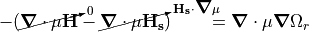
Also note that for permanent magnets (known ),
,  , and
implies
, and
implies  (Poisson Equation).
Even if is non-zero, magnetic vector potential may still be avoided
by utilizing reduced magnetic scalar potential,  .
Let
.
Let  be the component of the H-field due only to free current sources,
which is divergenceless and computable via the Biot-Savart Law.
When this is subtracted from H, we obtain an irrotational field,
be the component of the H-field due only to free current sources,
which is divergenceless and computable via the Biot-Savart Law.
When this is subtracted from H, we obtain an irrotational field,
 , which has a scalar potential defined by
 . The divergence is expressed as
 (Poisson Equation).
In the case
(Poisson Equation).
In the case  , this reduces to the Laplace Equation.
The differencing can cause loss in accuracy
but can be improved by using both reduced and total scalar potentials in different regions of the
problem [3].
, this reduces to the Laplace Equation.
The differencing can cause loss in accuracy
but can be improved by using both reduced and total scalar potentials in different regions of the
problem [3].
In summary, in the special case of zero current densities, magnetic H fields may also be represented as the (negative) gradient of scalar potentials, analogous to the situation in electric fields. However, in general magnetic B fields must be represented as the curl of vector potentials A, which happen to reduce to scalars in cases of 2D symmetry. Scalar potentials and vector potentials that reduce to scalars are distinct quantities though and should not be confused. In attacking a problem, note this:
Magnetic vector potential may always be used, but you may alternately use magnetic scalar potential (simpler) if current densities are zero.
Magnetic vector potential reduces to a scalar in 2D symmetries.
Non-constant permeability in 3D is more complex to solve with magnetic vector potential (and not currently handled by SIMION in this initial implementation) but can be handled with magnetic scalar potential.
Another complication is that in general can be a function of the B-field, but we are
using to solve for B. This complicated problem can be solved by self-consistent methods
(analgous to the treatment of non-linear forms of dielectrics). However, similar to how
the dielectric constants can be a function of the E field direction,
may also be a function of the B field direction (i.e. anisotropic), which the Poisson Solver in SIMION
presently does not handle. Another real possibility is that is a function of the past state
of the material (Wikipedia: Hysteresis), which we refer to as “hard” rather than “soft”
materials (Wikipedia: Coercivity); for example, forms of iron may be hard or soft.
See also Magnets and Hawkes and Kaser Principles of Electron Optics Volume 1, p.64 [4].
Magnetic Scalar Potential - Notes
Scalar magnetic potential is analogous to scalar potential in electric fields (i.e. voltage). The magnetic field vector is the negative gradient of scalar magnetic potential, just as the electric field vector is the negative gradient of electrostatic potential. SIMION can solve scalar magnetic potential using the Laplace equation in the same manner as electric potential is solved, and after doing so the magnetic field vector can be immediately obtained and used for particle trajectory solving. Unfortunately, not all magnetic fields can be expressed as scalars but rather as vectors, and the meaning of potential can be less intuitive with magnetic fields. Magnetic potential will be a scalar under certain conditions, such as when there is no current density in the domain modeled (and in a different way if the system has 2D symmetry). Beware also that, unlike the electrostatic case, magnetic pole surfaces do not generally have totally uniform magnetic potential across their surfaces, permeability not being infinite (see p. 2-10 of chapter 2 the SIMION 8.0/7.0 manual for a discussion of this). This presents a difficulty because surfaces of constant potential are normally used to define boundary conditions for the field solver. However, if permeabilities are infinite, or at least very large, and the region is sufficiently defined, then surfaces will have constant potential, and the boundary conditions are more readily definable in SIMION. Often, there is only one potential difference (i.e. between two poles) to define, and that potential can be scaled to give the desired field intensity between the magnetic poles.
Technically speaking, in SIMION, scalar magnetic potential is typically expressed in terms of a SIMION potential array. In SIMION, you can create a magnetic potential array just like you create an electrostatic potential array; a magnetic potential array can contain magnetic electrodes of arbitrary shape and that are assigned scalar magnetic potentials. You can then have SIMION refine it, in which case SIMION calculates scalar magnetic potential of the non-pole points by using the Laplace equation, just like for electrostatic electrodes. SIMION then uses these to compute magnetic fields in space. You may need to set the magnetic scaling factor so that the fields corresponds to real units of gauss. The calculated fields can even be non-uniform with fringing effects as seen in SIMION’s magnet examples (e.g. see screenshots of the 90 degree bending magnet, examples/magnet/mag90.iob, included in SIMION’s examples). This calculation does ignore any permeability and hysteresis effects. Another approach is to use the SL Tools utility to convert external field data directly into a SIMION potential array (without refining) of magnetic scalar potential or magnetic vector potential.
Defining magnetic scalar potential
The following is a simple example of creating a uniform magnetic field by way of a magnetic scalar potential array.
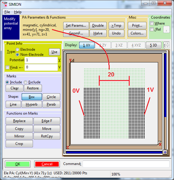
In particular note the annotations in red:
The array type is set magnetic.
The symmetry is set to 2D cylindrical or 2D planar, i.e. z=1 (not necessary, but this keeps memory usage small as noted previously).
The “ng” scaling factor is set to 20, which is equal to the distance between electrodes (mm). See p. 2-10 of the SIMION 8.1/8.0/7.0 manuals for the explanation of this crucial point and the limitations. The purposes of this scaling factor is just to get the units right.
SIMION 8.1 note: In SIMION 8.1, ng is not necessarily interpreted as grid units anymore but rather a distance in mm in the PA (as measured prior to any rescaling of an instance of that PA on the View screen > PAs > Positioning > scale). The PA cell size (prior to any rescaling) is by default 1 mm/gu in SIMION 8.1, and is always this value in SIMION 8.0, in which case there is no difference between measuring ng in grid units and mm distances. However, you can independently change the X, Y, and Z cell dimensions in the PA file as described in Anisotropically Scaled Grid Cells in SIMION.
Two electrodes of potentials V1 and V2 are drawn (here, V2 - V1 = 1 V). With the ng factor set as above, this will produce a field of (V2 - V1) gauss in the center (but this is approximate if there are fringe fields, as there are here because empty space is left at the top).
Verify the correctness of the magnetic field with SIMION Data Recording or by hovering your mouse over the volume.
This method is used by various examples in SIMION Example: magnet.
Note
This page is abridged from the full SIMION "Supplemental Documentation" (Help file). The following additional sections can be found in the full version of this page accessible via the "Help > Supplemental Documentation" menu in SIMION 8.1.1 or above:Magnetic Vector Potential PA’s in SIMION
Magnetic Vector Potential - Plotting