Using QuickField with SIMION
Introduction
QuickField is a finite element (FEM) field solver for many problem types, including in particular magnetic fields in 2D planar and 2D cylindrical symmetry. In also includes magnetic features such as non-linear and anisotropic permeability, DC, AC, and transient conditions.
This document describes how to interface the two programs, primarily to import magnetic field calculated from QuickField into SIMION, as well as other things like controlling QuickField from SIMION with the ActiveField API.
Topics in this document include:
Methods to import fields from QuickField into SIMION
Using a GUI toolbar.
Using the programming API.
Exporting from the QuickField GUI and and subsequently importing that into SIMION (this two-step approach is useful if SIMION and QuickField are installed on different computers).
Types of field import
Importing magnetic vector potential A from a QuickField .PBM file into a SIMION PA.
Importing Bx and By components of the B into from QuickField into two SIMION PAs.
Loading a QuickField finite element mesh into SIMION. This avoids interpolation onto a rectangular grid or PA.
Reading fields directly in real-time from QuickField using the QuickField’s ActiveField™ API. This eliminates any import step but is slower.
Viewing and plotting imported B fields.
Applying the B fields to particle trajectories with a short user program.
Drawing the QuickField finite element mesh in SIMION.
Other applications of using the ActiveField API within SIMION user programs to control QuickField.
You may want to first see the video summarizing the SIMION-QuickField integration: QuickField-SIMION Screencast.
Why Import?
Magnetic fields are important to SIMION because magnetic fields affect the particle trajectories (Lorentz Force Law) simulated by SIMION. Various types of instrumentation and mass spectrometers simulated by SIMION incorporate magnetic fields. So, we need to determine the magnetic field. Calculation of magnetic fields can be a little complicated, and SIMION has some magnetic capabilities (Magnets), but SIMION is more established in the area of particle optics and electric fields than magnetic problems, so there are times we may want to import magnetic fields from other packages, typically based on the finite element approach (FEM). You may prefer the FEM approach and the advanced and convenient magnetic capabilities provided in QuickField, so we ask how to export those fields from QuickField and import them into SIMION for particle optics handling and other analysis.
In SIMION we are typically most interested in ultimately knowing the
B field rather than the H field since the B field is used
for calculating particle motion by the Lorentz Force Law.
Nevertheless, it is also possible to import other
quantities like the H field or  if you so desire.
Moreover, we may actually import magnetic vector potential A,
which can be used to derive B indirectly.
if you so desire.
Moreover, we may actually import magnetic vector potential A,
which can be used to derive B indirectly.
SIMION and QuickField Versions
The QuickField integration is incorporated into SIMION 8.2.
Note: earlier versions of SIMION can also import fields, such as by using SIMION Example: field_array in SIMION 8.0/8.1 and the SIMION Example: contour (contourlib81) in SIMION 8.1, though it involves more work and you are more on your own.
These examples were tested in QuickField version 6.0.0.1508 but probably will also work in older and newer versions as well. If not, let us know, and necessary minor adjustments could be made.
SIMION-QuickField Toolbar
There is a toolbar that can be loaded into SIMION to provide convenient access to QuickField integration functions:
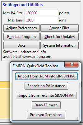
To access this toolbar, click Run Lua Program and on the
SIMION main screen and select the
examples\quickfield\qftoolbar.lua in the SIMION program folder.
Methods of Import
The basic approach
There is more than one way you may import magnetic fields into SIMION. Although you could import the B field vectors directly, it is suggested to instead import the magnetic vector potential A. (There is not a simple provision for exporting the magnetic scalar potential from QuickField.)
We also will normally import the field data as points on a uniform rectilinear grid rather than finite element mesh format since the former is conveniently represented as a regular SIMION potential array (PA) object, making it convenient and efficient to view and manipulate in SIMION.
Import Magnetic Vector Potential A
One means of importing the magnetic field into SIMION is to import the
vector magnetic potential A.
B can then be expressed in terms of A
by the equation  , which SIMION largely
takes care of for you.
For 2D problems, this A is convenient because only one dimension
of the A vector is non-zero (the z, or “azimuthal”,
component perpendicular to SIMION’s 2D xy plane), so it can be treated
as a scalar A, whereas B is a vector.
We can import A into a single SIMION potential array (PA),
whereas to import B likewise we would need two potential arrays,
one for each scalar component of the 2D vector.
For 2D cylindrical PA’s we will actually typically import
r*A, where r is the radial distance from the axis (y coordinate in SIMION).
(The use of the multiplying r factor under cylindrical symmetry
is a typical convenience, as noted on Magnetic Potential.)
, which SIMION largely
takes care of for you.
For 2D problems, this A is convenient because only one dimension
of the A vector is non-zero (the z, or “azimuthal”,
component perpendicular to SIMION’s 2D xy plane), so it can be treated
as a scalar A, whereas B is a vector.
We can import A into a single SIMION potential array (PA),
whereas to import B likewise we would need two potential arrays,
one for each scalar component of the 2D vector.
For 2D cylindrical PA’s we will actually typically import
r*A, where r is the radial distance from the axis (y coordinate in SIMION).
(The use of the multiplying r factor under cylindrical symmetry
is a typical convenience, as noted on Magnetic Potential.)
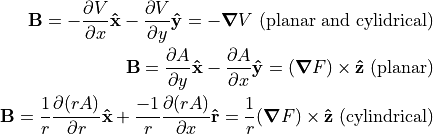
Now, SIMION magnetic potential arrays normally don’t store vector magnetic
potential A or r*A but rather a form of scalar magnetic potential V defined
as  .
Therefore, if we store A or r*A rather than V in the magnetic PA,
we need to slightly re-express the B that SIMION computes.
The necessary adjustment can be seen from the following equations.
The required adjustment is automatically taken care of by a SIMION utility
library we will use, so if you don’t follow that math don’t worry:
.
Therefore, if we store A or r*A rather than V in the magnetic PA,
we need to slightly re-express the B that SIMION computes.
The necessary adjustment can be seen from the following equations.
The required adjustment is automatically taken care of by a SIMION utility
library we will use, so if you don’t follow that math don’t worry:
QuickField can export so-called the Flux Function (F), defined as A for 2D planar (plane-parallel) symmetry and r*A for cylindrical (axisymmetric) symmetry, QuickField reports the values of r*A and A in units of Wb and Wb/m respectively, where 1 Wb (Weber) = 1 T m2 = 1010 gauss mm2 (SIMION units).
With SIMION 8.2 you can use the simple Field Functions Library (simion.experimental.field_array) utility library for computing B from A stored within a PA.
Import B Field Vector Components
Another approach would be to import  and
and  components of
the magnetic field.
The and components may be read directly
during the particle trajectory calculation
by having a SIMION
components of
the magnetic field.
The and components may be read directly
during the particle trajectory calculation
by having a SIMION mfield_adjust user program segment
consult either QuickField (slow) in real-time or a
finite element mesh exported from QuickField (faster).
Alternately, and may be stored in two
SIMION PA files, one for each component (e.g. “bx.pa” and “by.pa”),
although it’s often simpler to just store A in a single PA
as described previously.
This latter approach with bx.pa and by.pa is similar the SIMION Example: field_array
(SIMION 8.1).
All three approaches are also demonstrated in the SIMION Example: quickfield (bmag.iob).
Importing from QuickField into a SIMION PA - Using the Toolbar
The simplest way to import a QuickField field into a SIMION PA
is with the Import from .PBM into SIMION PA function on the toolbar.
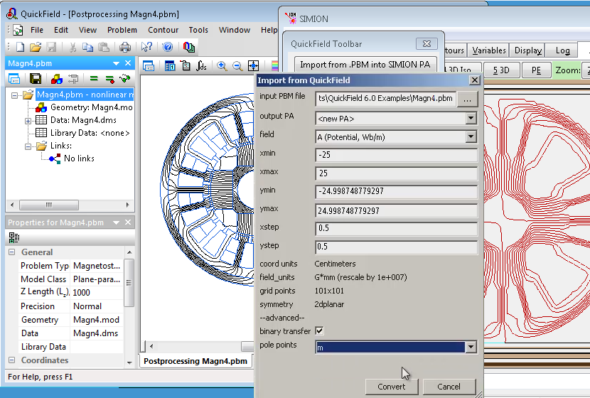
input PBM file- the QuickField PBM file to read the field from.output PA- the PA to import into. This can be a new PA (<new PA>) or an existing PA in SIMION’s memory.field- the field to import. Typically this is magnetic vector potential A, which is a scalar for 2D problems. You can alternately import the Bx and By vectors as two separate PA’s. Other field types can also be imported (e.g. temperature) if you needed.xmin,ymin,xmax,ymax- This is the boundary box in QuickField coordinates to extract the PA region from.xstep,ystep- This is the size of a PA grid unit in QuickField coordinates.coord units- This displays the coordinate units used by QuickField.field units- This displays the units used in SIMION for the selected field type. The units used in QuickField may be rescaled to SIMION units, such as using mm and gauss rather than tesla.grid points- This displays the number of points the SIMION PA will have in each dimension. This is typically (xmax-xmin)/(xstep) + 1 and (ymax-ymin)/(ystep) + 1.symmetry- This displays the symmetry of the QuickField problem, such as 2dplanar to 2dcylindrical. The SIMION PA created will have the same symmetry.binary transfer- If checked, data is transferred from QuickField into SIMION in binary rather than ASCII text format. Leave this checked. There should be no reason to uncheck it.pole points- Normally only the B field is imported, and pole material will appear invisible in SIMION apart from the field lines tracing boundaries. If “m” (permeability) is specified here, then anytime the permeability differs from 0 or 1, that point is made a pole point in the SIMION PA. This is optional and slows down the conversion some but makes the pole material easier to visualize.
It is alternately possible to import from a text file that was previously
exported from the QuickField GUI using the Import Text into SIMION PA
button on the toolbar:
input file- name of text file to import fromoutput PA- the PA to import into. This can be a new PA (<new PA>) or an existing PA in SIMION’s memory.column number- column in the text file containing the field value to import. Normally this is 3 since columns 1 and 2 are the X and Y coordinates and column 3 is the first field value.pole column number- optionally, column in the text file containing the magnetic permeability m (if any). Normally only the B field is imported, and pole material will appear invisible in SIMION apart from the field lines tracing boundaries. If “m” (permeability) is specified here, then anytime the permeability differs from 0 or 1, that point is made a pole point in the SIMION PA. This is optional and slows down the conversion some but makes the pole material easier to visualize.
Smaller grid cell (step) sizes provide more accuracy but also larger meshes. You proably want the grid cell (step) sizes in the PA to be roughly on the order of the size of your finite element cells since any larger loses accuracy and any smaller does not improve accuracy that much.
After importing the PA, you may want to open the SIMION View screen
and then click the Resposition PA Instance button on the toolbar
to reposition the PA instance within the SIMION workbench so that its
workbench coordinates are the same as in QuickField.
Exporting from QuickField Manually for Subsequent Import into a SIMION PA
The following process can be used to export field data from QuickField into a text file that SIMION can then later import into a SIMION potential array (PA). This is a two-step approach, which is more work than the previous method but may be required if QuickField and SIMION are not installed on the same computer. You can skip this section if you use the direct method described previously.
After solving the magnetic field in QuickField,
choose File > Export Field....
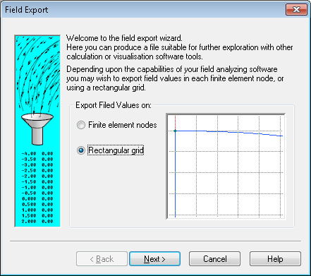
We want to use Rectangular grid in order to sample field data at points
on a uniformly spaced rectilinear grid, which is easy to store in a SIMION PA.
(Technically we might be able to utilize Finite element nodes, which exports
the data without any additional interpolation, but that format is not directly
storable in a SIMION PA, so we do not have the convenience and speed of the
visualization and interpolation capabilities afforded by PA’s.)
In SIMION we typical need to know the B field (rather than H field) since
the B field is used for particle motion (Lorentz Force Law).
So, we could either export the Flux Density values
(Bz and Br components in 2D
cylindrical or Bx and By components in 2D planar).
Alternately we could export a quantity like the Flux Function F, which
can be used by SIMION to derive the B field.
As described above, F (or A) is convenient because for a 2D (planar or cylindrical)
symmetry system, it represents the same information as the B but with a
scalar rather than 2D vector field.
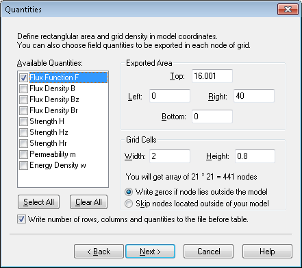
So, it is suggested to export F.
There is no harm in exporting additional columns of data, but we will
only really need F.
The rectangular volume to export is specified and the size of each grid unit. This will become the size of the PA and the size of a PA grid unit.
The grid cell size should probably be roughly the size of the triangles in your QuickField mesh, or perhaps a little smaller for increased accuracy. If the exported cell sizes are much larger then than the QuickField mesh triangles, you will likely introduce significant interpolation error (if it is ok to throw away accuracy, then why not calculate your QuickField mesh at lower resolution?). If the exported cell sizes are much smaller than the QuickField mesh triangles, then this increases memory usage and conversion time while likely not increasing accuracy significantly since the largest source of error in the field may be due to the size of mesh in QuickField itself rather than in the interpolation on the SIMION PA. If in doubt, you can experiment with different cell sizes and see how small the cells need to be to keep their effect on SIMION results within a desired threshold.
The option Write zeros if node lies outside the model is suggested rather
than Skip nodes located outside of your model.
Either way, the points will become zero in the SIMION potential.
However, if the Skip option is used, then the boundaries of the Exported Area
may be lost in the exported file if points with those extreme coordinates
are not inside the model.
Choose
Write number of rows, columns, and quantities to the file before the table.
This allows the SIMION conversion routine to quickly know the dimensions
of the arrays without counting rows and columns.
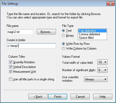
Specify the path of the output file to create (e.g. clicking Browse...).
Choose Text for File Type.
(The binary format is not supported. The binary format has the advantage of
being smaller but does not store the physical dimensions of the cell
or the symmetry, and Text should be ok as long as the file is not massive.)
The Tab delimited is recommended because it is the least ambiguous,
although Comma delimited also works well (with special heuristics if
the column name contains a comma like Field Gradient Gx,y (V/m2)).
Space filled may work in some cases (e.g. if
Join all title parts in a single string) but otherwise is not recommended
due to ambiguity in the format.
Choose all column titles (Quantity Notation, Verbal Description, and
Measurement Unit).
The Measurement Unit can be required for proper scaling of physical dimensions
and array values.
The Quantity Notation can be required for indicating the
type of symmetry used (x and y for 2D planar and
z and r for 2D cylindrical).
(It is possible, though there is little reason to, omit the
Verbal Description column.)
The value of Join all title parts in a single string doesn’t matter
unless you are using Space filled file type, in which case it should
(even must) be used.
It doesn’t matter if you select Write Row by Row or
Write Column by Column.
The conversion routine can handle either and will figure out which is used
automatically.
It is recommend to set the Values Format to be as accurate as possible
to avoid introducing numerical error in conversion.
For example, set Use scientific notation to Always and
Number of significant digits to 8 (maximum value).
The Total width of value field can be set to 10 (minimum value) since
it just adds extra surrounding spaces if larger.
Once you have exported the data file, you can import it into
SIMION using the Import from Text into SIMION PA function
on the SIMION-QuickField toolbar.
Importing from QuickField into a SIMION PA - Using the Programming API
It is also possible to import programmatically using user programs. You can skip this section if you instead use the toolbar GUI.
The library qflib.lua in SIMION Example: quickfield (in SIMION 8.1.2.8 or above)
can be used to convert QuickField PBM files or a text file exported from QuickField
into a SIMION potential array (PA).
It can be as simple as executing this from the SIMION command bar:
QF = simion.import 'c:/Program Files/SIMION-8.1/examples/quickfield/qflib.lua'
QF.convertqf{path='C:/Users/Public/Documents/QuickField 6.0 Examples/Magn4.pbm',
             output='A.pa'}
Alternately, you may want to add something like this to your workbench user program:
simion.workbench_program()
local QF = simion.import 'c:/Program Files/SIMION-8.1/examples/quickfield/qflib.lua'
function _G.regenerate()
  QF.convertqf{path='C:/Users/Public/Documents/QuickField 6.0 Examples/Magn4.pbm', output=1}
end
Now, anytime you enter regenerate() from the SIMION command bar within the
View screen, PA instance #1 will be automatically recreated
from the file Magn4.pbm.
This can be convenient if you need to edit the field in QuickField
and re-export it to SIMION multiple times.
You may need to resize the SIMION workbench (e.g. Min button on
Workbench tab)
or refresh the screen after regenerating.
The convertqf function has the following interface:
pa = QF.convertqf {path=path, output=output, col=col, polecol=polecol,
        xmin=xmin, ymin=ymin, xmax=max, ymax=ymax, xstep=xstep, ystep=ystep,
        binary=binary}
path- Path string of QuickField .PBM file to open. Ifnil, uses currently open file in QuickField.output- PA to write to. Can be a PA object, PA instance object, PA instance number, PA file name string, ornil(new PA in memory).col- Field to import. This is a field notation string (e.g. “A”), QuickField QfQuantity number (e.g. 0 is qfPotential) ornil(default).polecol- Field notation string (e.g. “m”), QuickField QfQuantity number, ornil(none). Optionally used to identify permeability. Points with permeability other than 0 or 1 are set to pole points in the PA, which helps in visualization.xmin,ymin,xmax,ymax- boundary box in QuickField units to extra PA region from.xstep,ystep- PA grid cell size in QuickField units.binary- boolean ornil(same astrue). Whether to transfer data in binary rather than ASCII text format. The default binary format is recommended.
Returns PA instance object.
The convert_file function has the following interface:
pa = QF.convert_file(infile, output, col, infile2, polecol, length_rescale)
Converts a QuickField text or binary file into a SIMION potential array (PA).
infileis that absolute or relative path to the QuickField text or binary file to import.outputcan be the absolute or relative path string to the SIMION PA file to write. Ifoutis a SIMION PA, PA instance object (e.g.simion.wb.instances[1]), or PA instance number (e.g. 1), then the field is imported into that existing object. Ifnil(the default), a new PA is created in memory.colis the column of from which values are imported. It can be a number (positive integer) column index or it can be a string that matches the description or notation string in a column header (e.g. “F”). If omitted, it defaults to 3. (Note that columns 1 and 2 are assumed to be coordinates.)infile2is absolute or relative path to the QuickField text file or binary to import for pole information. This is only used ifpolecolis specified.polecolis a column from which the pole/nonpole point type is determined. This is mostly intended to allow the user to better visualize the poles or allow particles to see the poles for splatting purposes. Values in this column that differ from 1 are assumed to be pole pieces and non-pole otherwise. The permeability (“m” column) may be suitable for this purpose, although some metals may have permeability of 1 (one workaround may be to change it to slightly different from 1 like 1.00001). If this columns is omitted, all points are assumed to be non-pole points.length_rescale- rescaling factor for length units in file (mm/file units). Used primarily for for binary files which specify the units used.
Returns PA instance object.
New PA object will be saved until out is nil.
If you are imporing Bx and By (or Bx and Br) field components directly, they you will need to convert the two arrays individually:
QF.convert_file('c:/temp/Magn2.txt', 'Bx.pa', 'Bx')  -- or 'Bz'
QF.convert_file('c:/temp/Magn2.txt', 'By.pa', 'By')  -- or 'Br'
or, again, if you prefer:
simion.workbench_program()
local QF = simion.import 'c:/Program Files/SIMION-8.1/examples/quickfield/qflib.lua'
function _G.regenerate()
  QF.convert_file('c:/temp/Magn2/Magn2.txt', 1, 'Bz')
  QF.convert_file('c:/temp/Magn2/Magn2.txt', 2, 'Br')
end
Warning: You should not ever Refine the PA imported into SIMION. The field is already solved, and Refining it will clear the field because the boundary conditions are not properly defined in the PA. In fact, SIMION will give a warning if you attempt to do so:
WARNING: This PA is not intended to be refined.
Refining will likely clear/corrupt it.
Details: This PA had been marked as not refinable (i.e. pa.refinable = false).
Some possible reasons for this are that the array is already refined but the
boundary conditions were removed from the PA or the array is being used in an
unconventional way to hold data not understood by Refine."
If desired, you can enable X and/or Y mirror planes on the PA
using the Set function on the Modify screen (or via Lua code).
If this is done, you should only import the positive (first) quadrant
into the PA and then enable mirror planes to obtain the fields in the
other quadrants.
Reading Fields Directly in Real-Time through ActiveField
SIMION can optionally read fields directly in real-time from
a running QuickField program using the
QuickField’s ActiveField™ API,
rather than converting the field to a uniform grid or PA.
An example of this is commented out in the bmag.lua
in SIMION Example: quickfield.
This approach is convenient and accurate because it avoids interpolation
but is is also relatively slow if doing a lot of particle tracing.
simion.workbench_program()

-- Load the B field reader.
local QF = simion.import 'qflib.lua'
local bfield = QF.field_from_qf(
    'C:/Users/Public/Documents/QuickField 6.0 Examples/magn2.pbm','',  1)

-- optionally plot the field vectors
CON.plot{func=bfield, mark=true, npoints=20, z=0}

-- optionally allow particles to see the field
segment.mfield_adjust = simion.experimental.make_mfield_adjust(bfield)
Reading Fields (or Geometry) Directly from the QuickField Finite Element Mesh
SIMION can optionally read the QuickField finite element mesh directly, rather than converting the field to a uniform grid or PA. It is possible to load this finite element mesh into SIMION and have SIMION draw it and/or interpolate fields from the finite element mesh. This approach avoids accuracy loss of interpolating onto a rectangular grid. No PA is involved, although you might optionally also import a PA for visualization purposes. The finite element can be loaded directly from the running QuickField program or from a text file of the finite element mesh exported from the QuickField GUI.
You can use the Draw FE mesh button the toolbar to draw the mesh:
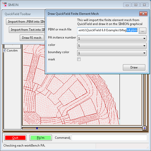
This can also be helpful if you just want to draw the boundary of materials rather than individual finite element cells:
(Use the “Del” button on the Particles tab to clear the drawing.)
An example of loading the mesh, drawing the mesh, plotting the field, and
making it visible to particles from within a user program
is commented out in the bmag.lua in SIMION Example: quickfield.
simion.workbench_program()

-- load the finite element mesh
local QF = simion.import 'qflib.lua'
local mesh = QF.read_mesh('magn2-fe.txt', 1)
local bfield = QF.mesh_to_field(mesh)

-- optionally draw the mesh
QF.draw_mesh{mesh=mesh}

-- optionally plot the field vectors
CON.plot{func=bfield, mark=true, npoints=20, z=0}
--CON.plot{func=bfield, mark=true, npoints=20, y=0}
CON.plot{func=bfield, mark=true, npoints=20, x=300, color=6}

-- optionally allow particles to see the field
segment.mfield_adjust = simion.experimental.make_mfield_adjust(bfield)
Viewing the Fields in SIMION
If you imported a PA, you can add it to the workbench (View screen) and use the PE and Contour functions in the usual way to plot the fields:
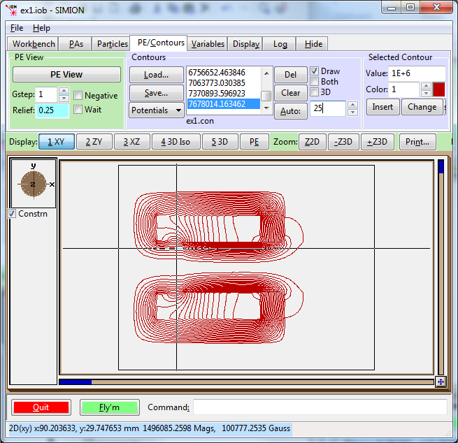
Note that the potential contours and the values with label Mags in the status
bar are of the F function, with units of
gauss mm2 ng (F=A*r, for 2D cylindrical PA’s) or gauss mm ng
(F=A, for 2D planar PA’s). (The unitless magnetic scaling factor ng
is normally 1, or at least the conversion library makes it so.)
Beware that any B values displayed in the status bar or Data Recording are
actually  , which is probably not really what you want.
Also any values of
, which is probably not really what you want.
Also any values of  displayed are
  ,
which are the same as for 2D planar symmetry but are
,
which are the same as for 2D planar symmetry but are
 for 2D cylindrical symmetry.
In the screenshot above, the value is about 100777
gauss*mm but since this is 2D cylindrical symmetry it must be divided by
the radial distance y=29.7 mm to obtain about 3390 gauss as the value
for .
for 2D cylindrical symmetry.
In the screenshot above, the value is about 100777
gauss*mm but since this is 2D cylindrical symmetry it must be divided by
the radial distance y=29.7 mm to obtain about 3390 gauss as the value
for .
Plotting with the Contour Library
Besides PE/Contour functions, you can use the SIMION 8.1 contour library (SIMION Example: contour). This will plot vector fields and is especially useful if importing the B field vectors directly since there you don’t have a scalar potential to plot or if you import the fields without using a PA (e.g. importing a finite element mesh as shown previously).
simion.workbench_program()
local B = simionx.experimental.field_array{Bx=1,By=2}
segment.mfield_adjust = B.mfield_adjust

local CON = simion.import 'c:/Program Files/SIMION-8.1/examples/contour/contourlib81.lua'
CON.plot{func=B.bfield, mark=true, npoints=20, z=0}
print('TEST', B.bfield(10,0,0))  -- read single point (mm, gauss)
The bfield property on the field array object is a function
representing the B field, suitable for plotting or testing,
and works with field arrays created from B and A.
Some of the examples in SIMION Example: quickfield utilize the
contour library.
Applying the B Field to Particles
The particles will not properly see and interpret the B field
in the PA of magnetic vector potential.
They are not aware that the values in the PA are not scalar magnetic potential
but rather vector magnetic potential.
In fact, if you used Data Recording to record the B field the particles
see, you will observe it is not correct.
We can rectify this with a short workbench user program that defines an
mfield_adjust segment to override the B field with one properly
interpreted from the PA (a future update to SIMION will eliminate the
need for this user program, but for now this is the quick adjustment).
If you have a 2D planar PA storing the z component of
magnetic vector potential  , then
just attach the following short user program to the SIMION workbench.
(As usual, click
, then
just attach the following short user program to the SIMION workbench.
(As usual, click User Program... from the Particles tab,
paste the code into the file, and save.)
simion.workbench_program()
local A = simion.experimental.field_array{Az=1}
segment.mfield_adjust = A.mfield_adjust
If this is a 2D cylindrical PA storing r A, then
replace the name Az with rA:
simion.workbench_program()
local A = simion.experimental.field_array{rA=1}
segment.mfield_adjust = A.mfield_adjust
If you have two PAs containing the Bx and By components of the B field, do something like this:
simion.workbench_program()
local B = simionx.experimental.field_array{1,2}
segment.mfield_adjust = B.mfield_adjust
Note: the above assumes PA instance numbers 1 and 2 (as displayed in the PA Instances list on the PAs tab) represent the Bx and By field components respectively; if not, change the numbers in the code accordingly. Likewise for the other examples above.
(Note: The Field Functions Library (simion.experimental.field_array) library requires 8.2-2014-04-12 or above.)
You can now define particles, Fly them, and Data Record in the usual way
in SIMION.
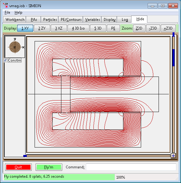
Below shows the vmag.iob example in SIMION Example: quickfield.
For simplicity of demonstration, only a single 10 keV electron is flown.
Note that the field is quite strong and the particle roughly follows the
contour lines of rA (which also follow B field lines)
with additional helical motion that is only visible at higher particle energies.
(This example is a bit fictitious since the region the particle is flying, apart from
the small gap, is actually solid metal, but it suffices for demonstration, and if needed
we could force particles to splat on touching metal as described later.)
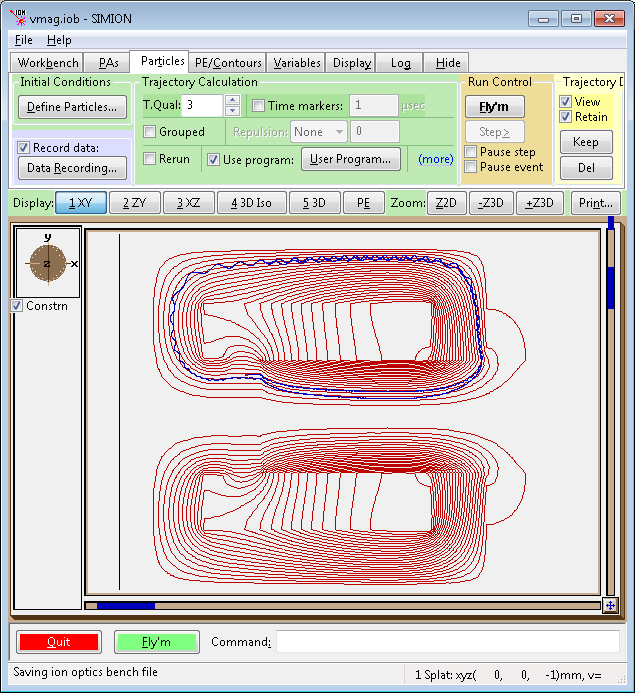
Fig. 30 2D view of flux function (F=rA) contour lines (red) and particles (blue).
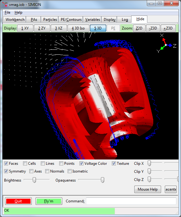
Fig. 31 3D view (SIMION 8.2) of magnetic vector potential contour surfaces (red) and particles (blue), as well as contour library field vector planes (white and black).
Program Templates
The toolbar has a button Program Templates for displaying
useful user program code you can copy and paste into your own
user program.
This allows you to quickly add necessary code.
Accuracy and Other Conversion Tips
Checking the Conversion
It is strongly recommended to confirm that the field imported into SIMION is approximately the same as the field in QuickField in case some simple error was made in the conversions of physical dimension units, magnetic potential units, symmetry, or poor grid cell size. The rule in SIMION and any simulation program is “always be suspicious.”
First make a visual check. Draw contours in SIMION to see the field and ensure it looks qualitatively similar, as they are in the figures above and below. Also hover your mouse over the field in SIMION to measure physical dimensions to ensure they are the same as in QuickField.
Note that SIMION dimensions are by default in units of mm.
Although not required, it can be convenient to set Length units to
Millimeters in the QuickField
problem properties so that both programs display in the same units.
Check the value of the B field on at least one point in both programs
and compare.
The Local values tool on the Postprocessing window in QuickField can be
used to read the field value at the given point by clicking on the point in the
graphical window or typing it exactly in the left pane (e.g. “9 3” cm for x and r).
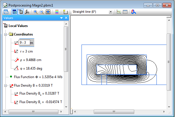
In SIMION, you can add something like this to your workbench user program:
simion.workbench_program()
local A = simion.experimental.field_array{rA=1}
print('TEST', A.bfield(90, 30, 0))
or just copy and paste this one-liner on the command bar:
=simion.experimental.field_array{rA=1}.bfield(90, 30, 0)
(Be careful to specify “rA” or “Az”.)
The B field (x, y, and z components) will display in the status bar
(or remove the “=” and wrap it inside a print( ) command like previously
to write it to the Log window tab).
If flying particles, also check that the particles see that correct B field.
Define an mfield_adjust segment as described previously,
fly some particles and use the standard Data Recording
features to measure the B field observed by the particles at some
position (convenient places are Ion's Start, Ion's Splat and Crossing Plane.
This confirms that everything is operational.
Some difference in the QuickField and SIMION field is expected due to
the differences in interpolation.
This error can be reduced by decreasing the Grid Cell Width
and Height values in the QuickField export, as discussed previously.
Pole/Non-Pole PA Point Types and Particle Splatting
The default is to import the field without any information of pole/non-pole
point types.
So, you will not see the poles during visualization (apart from the contours),
nor will particles see the poles for splatting purposes
(unless of course you have an
electrostatic PA or user program causing the splatting).
If you want the point type set in the PA, you may be able to infer this from
the permeability (m) value exported by QuickField by passing m as the
fourth argument to the convert function.
For further details, see the description of the pole col in the conversion.
Converting Magnetic Vector Potential to Magnetic Scalar Potential
You may for some reason want a PA with magnetic scalar potential rather than magnetic vector potential. There does not appear to be an option of exporting the magnetic scalar potential directly from QuickField. It is not even always possible to do this uniquely on the whole domain, like when you have current sources.
The SIMION function simion.experimental.spotential_from_vfield()
(see spotential_from_bfield.iob in SIMION Example: magnetic_potential)
may be used to convert a known B field to magnetic scalar potential
(over at least some of the domain) by integration.
This is not normally recommended and may introduce some loss in
accuracy too but can be done.
Controlling QuickField from SIMION
The QuickField “ActiveField” API can be called from SIMION user programs
via the COM (luacom) interface to control QuickField from SIMION
for various purposes, not just importing.
An example activefield.lua is included in SIMION Example: quickfield.
-- Load model.
local qf = luacom.CreateObject("QuickField.Application")
local prb = qf.Problems:Open(
    "C:/Users/Public/Documents/QuickField 6.0 Examples/magn1.pbm")
print(prb.Solved)
if not prb.Solved then
    print ('cansolve', prb.CanSolve)
    if not prb.CanSolve then error "cannot solve" end
    prb:SolveProblem()
end

print(prb)
print(qf)

prb:AnalyzeResults()

local result = prb.Result

print('units', prb.LengthUnits)
print('coord', prb.Coordinates)
print('ptype', prb.ProblemType)
print('ptype', prb.ProblemType1)
print('result', result)

local fp = result:GetLocalValues(qf:PointXY(0,40))
print('p', fp.Potential) -- Wb/m
See the ActiveField documentation in the QuickField help file for more details.
Ordering
Contact SIS for any help on the integration between QuickField and SIMION or if you want a quote and demo version of these softwares.
Future Improvements
Ideas includes
It is planned for PA’s to know about magnetic vector potential directly without needing to attach the extra piece of user code. [TODO82]
Add more ActiveField API examples.
Changes/History
2014-08-09: fix imported magnetic cylindrical scalar potential values in PA values being 1000x too small due to older QuickField versions wrongly reporting units “A (Wb/m)” rather than “F (Wb)”. Works arounds problem by correcting units.
2014-03-08: initial version, D.Manura