Earnshaw’s Theorem
Earnshaw’s theorem states that “A charged particle cannot be held [statically] in a stable equilibrium by electrostatic forces alone.” (Griffiths, p.115)
Another way to express this is that the Laplace Equation has no
solution  with local extrema (minima or maxima) in free space.
may, however, have unstable saddle points
(Wikipedia: Saddle_point) such as in the center of a multipole
(like SIMION Example: octupole shown in Figure 1).
Local extrema can, however, exist on the electrodes (boundary conditions).
If there is space-charge (Poisson Equation),
local extrema can occur near the space-charge
with local extrema (minima or maxima) in free space.
may, however, have unstable saddle points
(Wikipedia: Saddle_point) such as in the center of a multipole
(like SIMION Example: octupole shown in Figure 1).
Local extrema can, however, exist on the electrodes (boundary conditions).
If there is space-charge (Poisson Equation),
local extrema can occur near the space-charge
 (Figure 2).
Earnshaw’s theorem can be understood by the fact that under the
Laplace equation, the potential at a point is basically the
average of the potentials of the points surrounding it:
 for a sphere surface S of area A centered at
  (Griffiths, p. 113).
This equation can be observed in SIMION [1] and it is
likewise observed in the finite difference equations
(“refining equations” in the “Computational Methods” appendix of the
7.0-8.1 SIMION User Manual).
(Griffiths, p. 113).
This equation can be observed in SIMION [1] and it is
likewise observed in the finite difference equations
(“refining equations” in the “Computational Methods” appendix of the
7.0-8.1 SIMION User Manual).
This theorem has implications on ion traps, which hold particles in place but do so by other means such as magnetic or RF electric fields. Purely electric fields can also trap dynamically moving charged particles (see Electrostatic Trap), which is not a violation of Earnshaw’s theorem.
Some examples of SIMION computed fields illustrating Earnshaw’s theorem are shown in the Figure 1. Local extrema in free space are indeed never observed, at least in the absence of space charge like in Figure 2.
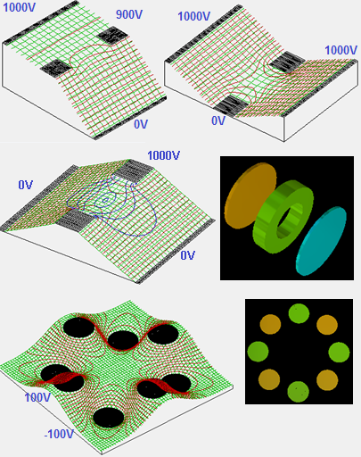
Fig. 80 Figure 1: Various examples of electric fields calculated in SIMION. Potential energy surfaces are in green. Potential contour lines are in red. Contour lines of E-field magnitude are in blue. 3D views of the two geometries used are shown on the right. Local minima are never observed in free space, in agreement with Earnshaw’s theorem, though (unstable) saddle points are observed, and minima do exist on electrode surfaces (including ideal grids). These models are taken from SIMION Example: tune and SIMION Example: octupole (SIMION 8.0/8.1).
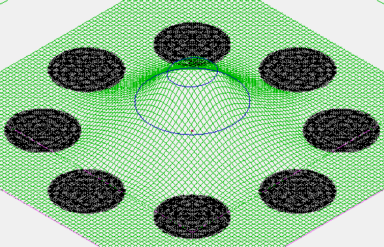
Fig. 81 Figure 2: Grounded rods with space-charge in the center. Potential contour lines in blue. The space-charge forms a local extremum in the potential energy surface. This model is taken from SIMION Example: poisson (octupole_sc) (SIMION 8.1), where the space-charge is formed from an ion beam. The potential is solved using the Poisson Solver in SIMION.
Neutral Particles
Neutral particles with a dipole are affected by electric fields. How does Earnshaw’s theorem apply here? Neutral particles can be either “low-field seekers” or “high-field seekers.” In free space, the magnitude of the electric field can have a local minimum (e.g. see blue lines in Figure 1) but not a local maximum.
“In contrast, the electric field strength can have a minimum in free space (note that the Earnshaw theorem does not allow for a maximum), and molecules in low-field seeking quantum states, that is, in quantum states with a negative effective dipole moment, can thus be trapped with static electric fields.” (van de MeerakkerBethlem2012)
“…we shall show below that the stable levitation and trapping of a neutral polarizable object, which is a high-field seeker, is generally impossible in an arbitrary electrostatic field configuration…. Some known ways to evade Earnshaw’s theorem and, thereby, to construct a truly stable trap for charged particles or for neutral particles are as follows: … (iv) to use the low-field seeking property of neutral diamagnetic objects to levitate them in strong inhomogeneous magnetic fields.” (MinterChiao2007)
Footnotes
[1] To verify this equation in practice (under SIMION >= 8.1.1), open SIMION Example: octupole, fast adjust electrodes #1 and #2 to 100 and -100 V respectively, and then enter the following (all on one line) into the bottom SIMION command bar:
local INT = require 'simionx.Integration';
local R = 100; local area = 4*math.pi*R^2;
local x0,y0,z0=150,50,0;
local co = INT.montecarlo_integrate{
  func=function(x,y,z) return simion.wb:epotential(x,y,z)/area end,
  shape=INT.sphere(x0,y0,z0, R)};
repeat local result, result_stdev, count, is_end = co();
print(result, result_stdev, count, is_end) until is_end;
print(simion.wb:epotential(x0,y0,z0), '<-- expected')
which uses simionx.Integration - Numerical integration routines and simion.wb. The output demonstrates equality (within numerical accuracy of this array and integration) for both sides of the equation:
...
-2.1833243254334     0.0013340750177746      131072  true
-2.1856750962739     <-- expected
Note: for large R, the difference between both sides may provide an order-of-magnitude estimate of the numerical error in the field.
See Also
MinterChiao2007. Minter, S. J.; Chiao, R. Y. “Can a charged ring levitate a neutral polarizable object? Can Earnshaw’s theorem be extended to such objects?” Laser Physics. volume 17, issue 7, year 2007, pages 942-947. doi:10.1134/S1054660X07070079.
van de MeerakkerBethlem2012. van de Meerakker|, Sebastiaan Y. T.; Bethlem, Hendrick L.; Vanhaecke, Nicolas; Meijer, Gerard. “Manipulation and Control of Molecular Beams” Chemical Reviews. volume 112, issue 9, year 2012, pages 4828-4878. doi:10.1021/cr200349r.